Category Archives: Theory

Is Your System Broken?

The Ultimate Test of Efficacy: Time

At Futures Truth, we focused on one thing: walk-forward results across hundreds of trading systems. Back then, the industry was unrecognizable compared to today—if you can even call what exists now an “industry.”

Just this morning, I was reminiscing about vendors who sold strategies for upwards of $5,000. Those packages usually consisted of a set of rules (disclosed or not) and a rudimentary DOS-based program to generate simple charts and next-day orders. This was well before the heyday of TradeStation; those days are gone forever, for better or worse.

Back then, if a system performed well in walk-forward analysis, it earned a ranking. In those days, a Futures Truth ranking meant something. Sometimes, however, that ranking felt like a curse. Critics even argued you could “fade” a top-ranked system and make more money by taking the opposite trade. The reality is that many of those legendary “Top Ten” systems—built for a different era—simply wouldn’t survive in today’s markets.

Side Bar:  There are still services such as Striker and The Collective that still monitor trading systems.  Striker only shows real execution, which is mostly a good thing – real execution costs are shown.  But so is broker error.  Heck, we are all human and we all make mistakes.  Striker is upfront with this, and they state they will do the best they can – execution can be a beast. 

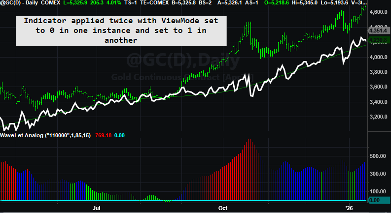
Speaking of execution – The Sunday Evening Gap

A Traders Nightmare. Most likely Trend Followers were short during the huge gap here!

 Imagine, having a stop order in crude oil on a Sunday evening when the market opens thousands of dollars through your stop.  If a system derived position is short the broker’s only directive is to GET OUT – no matter what, at the first off ramp.  The above chart shows a single contract slip on crude futures at the genesis of the Iran War.

The Million-Dollar Question

The second most common question I was asked at Futures Truth was: “How do I know if the system I’m trading is broken?”

Can you guess the most common one? “If it were your money, which system would you trade?”

We never answered that one directly; there was never a simple black-and-white answer. But the second question—the one about “broken” systems—usually surfaced when a trader was deep in a drawdown.

Seasoned traders know that systems ebb and flow; drawdown is simply the “tax” we pay to play the game. Others, however, get “married” to a system and stick with it until “death do us part.” My standard response back then was always:

“Is your current performance still within the boundaries of the backtest?”

In other words, has the system exceeded its historical maximum drawdown by a meaningful margin? Does the current real-time performance look like other “rough patches” in the historical equity curve? If the answer was yes, the trader would usually give it a little more room.

Into Unexplored Waters

Those were simpler days, but the core problem remains: we cannot see the future. No forward analysis can tell you with certainty what a trading system will do next. What it can do is tell you when the system has moved into “unexplored waters.” Once you know that, the decision to stay, abandon, or pause becomes much easier.

All trading systems oscillate between success and failure. If a system has a genuine technical edge, that edge may eventually reassert itself—provided you have the time and capital to wait. But most traders don’t have unlimited resources.

Recently, the market activity surrounding the Iran conflict has pushed many systems into intense drawdowns. The same old questions have reared their heads again. This time, however, I wanted to provide a more empirically derived analysis. I’ve developed a disciplined approach to measuring risk and reward that moves beyond “gut feel.”

To illustrate, I pulled a system off my shelf that I originally designed for retail consumption back in June 2018. Here is how it’s currently holding up:

Hypothetical Results: Before and after development.

The Profit Mirage

This is a mean-reversion approach. I remember thinking back in 2018: How much longer can this bull market continue? With that in mind, I utilized a simple regime filter. After just a few weeks of trading later that year, I genuinely thought the system might be broken. The market spent a large portion of that fall and winter below its 200-day moving average, and shorting simply wasn’t working.

The system then went dormant for a long stretch, finally “waking up” at the height of the pandemic. Had you stuck with it, you would be up significantly today (though we stopped trading right at the onset of the pandemic).

But here is the catch: Profit, by itself, is not enough to determine if a system is broken. As long as they are making money, most traders never bother to peek below the surface. This system would likely be sitting near the top of the Futures Truth rankings today. But let’s dive in and see how it actually performed on its “test of time.”

Test 1 – Baseline Projection

Baseline projection based on in sample average monthly return.

Is Outperformance Always a Good Thing?

Looking at the chart above, you see a steep deviation below the baseline initially, followed by a rocket-ship move to the upside. By late 2025, the actual equity is sitting way above the red dashed expectation line.

Most traders would see this and think they’ve struck gold. “Isn’t this what we want—a strong positive deviation?” they’d ask.

In a world of simple “bottom-line” thinking, the answer is yes. But in the world of professional algorithmic trading, this chart is screaming a different story. To a seasoned developer, deviation is deviation. Whether it’s to the upside or downside, moving this far away from the “expected” path suggests that the strategy’s original statistical model is no longer in control.

When a system starts generating 190% of its expected return, it’s often because it has inadvertently stepped into a high-volatility regime it wasn’t designed to navigate. If the “upside” is this aggressive, you can bet the “downside” risk has scaled right along with it.

Test 2:  Monte Carlo Analysis on Walk Forward

Return and Drawdown sitting on the tails.

The Statistical Reality Check

To understand why I called this system “Degraded” despite the profits, we have to look at the Monte Carlo Walk Forward distributions. This is where we compare real-time performance against thousands of simulated “alternate realities” based on the system’s history.

1. The Equity Distribution (The Good News… or is it?)

In the top chart, our actual forward equity of $67,575 (the dashed red line) sits at the 97th percentile.

  • Interpretation: Out of 1,000 possible outcomes, the system performed better than 970 of them. While this looks great, being this far out on the “tail” of the distribution suggests we are no longer operating in a normal environment.

2. The Drawdown Distribution (The Warning)

The bottom chart is the real story. The actual worst drawdown reached $18,588, placing it in the 98th–99th percentile of severity.

  • The Comparison: The median expected drawdown was only $8,125.

  • The Verdict: We have blown past the 90th percentile of $13,611 and are deep into the “danger zone.”

The Bottom Line

When a system hits the 97th percentile for gains but simultaneously hits the 99th percentile for drawdown stress, the math is telling you that the character of the strategy has changed. You aren’t just trading a system in a “rough patch”—you are trading a system that has moved into a risk regime it was never built to survive. This is the “evidence-based framework” I mentioned earlier. Without these charts, you’re just guessing. With them, you have the data to justify stepping aside.

The Verdict: Test 3 – Overall Assessment

This is where the “gut feel” ends and empirical analysis begins. The following commentary is generated by my new software; a quasi-expert system designed to pair raw statistical results with descriptive, actionable interpretation.

Status: DEGRADED

Risk Assessment: CRITICAL RISK

Incubation/Trading Readiness Score: 4 / 8

Overall Assessment: Degraded
Risk Assessment: Critical Risk
Incubation/Trading Readiness Score: 4 / 8
Return delivery is running ahead of baseline: expected annual return is 18% versus actual annual return of 34% and expected annual gain of $4,477 compares with actual annual gain of $8,536. However, that stronger return delivery has come with a less stable path and/or materially heavier risk than history would suggest. Risk is materially worse than the historical profile: actual worst drawdown of $18,588 is 2.670 times the historical drawdown of $6,962. Risk conditions are now in the Critical Risk range. The realized monthly path is poorly aligned with the baseline, based on monthly equity correlation of 0.960, projection RMSE of $21,789, normalized RMSE of 4.867, and path wander ratio of 0.621. Correlation still describes directional similarity, but RMSE and path wander ratio show how far the realized path has wandered from projection over the same window. Monte Carlo context is cautionary: actual forward equity is $67,575, gain percentile is 97% (near the top of the simulated distribution), and drawdown percentile is 99% (in the worst decile for drawdown stress). Taken together, the system shows meaningful deterioration in incubation.

A readiness reading of 4 out 8 indicates this system right now has degraded to a point where caution and I mean extreme caution should be used in your decision to trade this strategy.  The major factors influencing rating are:

  • Return Attainment:   1.907 – — This indicates the system has achieved 190.7% of its historically expected return during the incubation/trading period. In practical terms, the strategy is generating returns at nearly twice the pace implied by its historical baseline.
  • Path Wander Ratio: 0.621 — This indicates that the actual equity path is deviating from the projected path by a meaningful amount relative to the total expected move over the incubation/trading period. Put simply, the system is not wildly off course, but it is no longer tracking the historical baseline tightly.
  • Drawdown Stress: 2.67 — This indicates that the actual worst drawdown has expanded to roughly 2.7 times the level suggested by the system’s historical baseline. Put simply, the strategy may still be generating return, but it is doing so while absorbing far more pain than its historical profile would justify.

Hindsight is always 20/20, and it is easy to say now that you should have stuck with the system. But with a large sample of out-of-sample trades showing this degree of deterioration, if I had to choose between staying with it, abandoning it entirely, or temporarily shutting it down, I would probably step aside and wait for conditions to settle down. Remember, not trading is an algorithm too.   Having the right tools to make this kind of decision is paramount, because they give you an evidence-based framework for explaining and defending your reasoning.

The Power of Incubation: Is Your Best System Collecting Dust?

How many systems do you have sitting on your shelf? I personally have at least a hundred, probably more. In this business, a little dust is not always a bad thing.

Figuratively speaking, the more “dust” a system has collected, the more real-time incubation it has endured. And that gives you something far more valuable than any backtest: pure, unadulterated out-of-sample evidence.

Seeds Waiting to Be Planted

Algorithmic trading development rarely produces just one system. It creates a trail of offshoots—versions that may have looked unremarkable or even mediocre during the initial build. Yet many of these forgotten systems are really just seeds waiting for the right environment.

When you revisit them months or even years later, you may find that a strategy which struggled in 2022 has bloomed into a powerhouse in 2026. Without a framework to measure that growth, you would never know.

Why You Need an Incubation Framework

Most traders revisit old systems by simply eyeballing an equity curve. An incubation framework goes much deeper by providing:

Historical Context: Does the dusty system’s recent performance still match its original DNA?

Regime Readiness: Has the market finally moved into the regime this offshoot was designed for?

The Go/No-Go Signal: A quantitative way to decide whether a seed is finally ready to be moved from the shelf to the server.

TS-SystemChecker software

TS-System Check Control Panel

A Tool Built for the Journey

I built TS-SystemChecker because, after decades at Futures Truth and years of developing my own strategies, I needed a better way to cut through the emotional fog that surrounds system evaluation.
I didn’t design TS-SystemChecker to be a black box or some kind of get-rich-quick shortcut. I built it because, after decades at Futures Truth and years of developing my own strategies, I wanted a better way to cut through the emotional fog that surrounds system evaluation.

Whether you are a retail trader focused on refining one core system, or a developer like me with a shelf full of offshoots, this framework was built for that journey.

For the specialist: If you have one system you live and die by, the deep-dive analysis helps define its boundaries of truth. You can begin to see whether a drawdown is simply part of the system’s normal character or evidence of something more structural.

For the portfolio manager: If you are tracking a library of ideas, the Batch Analysis feature helps you monitor many systems at once. Import the trade files, review the evidence, and identify which seeds may finally be ready to move from the shelf to a live account.

Looking Beneath the Surface

At the end of the day, this is why I built TS-SystemChecker. Traders need more than opinions, hope, or fear. They need a framework grounded in evidence.

That is the real purpose of this tool: not to make decisions for you, but to help you make better ones.

TS-SystemChecker Batch Mode

Reverse-Engineering a Trading Indicator with AI

From Raw Wavelet Code to a Trading Tool with More Knobs Than Anyone Was Turning

The Indicator I Thought I Understood

A client sent me a trading indicator they had just started using.
It was short. Clean. About a page of code.

I’m not entirely sure where it originated, but it had the unmistakable feel of something machine-generated — technically sound, compact, and largely undocumented.

Their usage was simple:

  • Plot one line
  • Look at its slope compared to one bar ago
  • Go long or short accordingly
{---------------------------------------------------------
Causal True ? trous Wavelet Indicator
---------------------------------------------------------}
Inputs:
UseD1(true),
UseD2(false),
UseD3(false),
UseD4(false),
UseD5(false),
UseD6(false),
ColorBarsByTrend(true),
InvertTrendColorMap(false), // optional flip if colors look reversed
TrendColor(green), // used only if ColorBarsByTrend = false
DenoisedColor(white),
ResidualColor(red);
Vars:
Price(0),
c0(3.0/8.0),
c1(1.0/4.0),
c2(1.0/16.0),

...
...
...
// --- Step 1: Current price ---
Price = Close;
// --- Step 2: A0 is raw price ---
A0 = Price;
// --- Step 3: Causal ? trous B3-spline filter (past bars only) ---
A1 = c0*A0 2*c1*A0[1] 2*c2*A0[2];
A2 = c0*A1 2*c1*A1[2] 2*c2*A1[4];
A3 = c0*A2 2*c1*A2[4] 2*c2*A2[8];
A4 = c0*A3 2*c1*A3[8] 2*c2*A3[16];
A5 = c0*A4 2*c1*A4[16] 2*c2*A4[32];
A6 = c0*A5 2*c1*A5[32] 2*c2*A5[64];
// --- Step 4: Details ---
D1 = A0 - A1;
D2 = A1 - A2;
D3 = A2 - A3;
D4 = A3 - A4;
D5 = A4 - A5;
D6 = A5 - A6;
// --- Step 5: Trend ---
Trend = A6;
...
...
// --- Step 7: Residual ---
Residual = Price - Reconstructed;
// --- Step 8: Plot ---
Plot1(Trend, "Trend");
Plot2(Reconstructed, "Denoised");
Plot3(Residual, "Residual");
Wavelet a trous snippet

They were using a single configuration — effectively listening to just one component of the indicator: Trend. And to be fair, it mostly worked. The trouble only appeared when the Residual (what ever that is) was plotted alongside it. Because it lived on a very different scale, it crushed the display and made the indicator look unusable. See the section at the bottom of this post for how to fix that. Other than that, nothing was actually “broken.”

That behavior was also an early clue that the code itself was likely AI-generated. If you’ve worked with John Ehlers–style indicators, you may recognize the fingerprints of Digital Signal Processing here: fixed coefficients, repeated smoothing, and the output of one calculation feeding directly into the next in a cascading fashion. Those are classic DSP techniques — powerful, but easy to mislabel or oversimplify when dropped directly into a trading context.

In hindsight, the breadcrumbs were right in the header: wavelet and à trous. Even if you’ve never heard those terms, you can paste them into an AI chat and ask, “What does this mean?” That won’t instantly tell you how to trade it — but it will give you the vocabulary and the map so you’re not reverse-engineering in the dark. From there, the real work becomes translating the math into something a trader can actually see and use.

What is a wavelet à trous?

A wavelet à trous (“with holes”) method is a signal-processing technique that breaks a data series into multiple layers, each representing a different time scale. It does this by repeatedly smoothing the data while spacing the filter farther apart at each step, without downsampling the signal.

The result is a set of detail layers (short-term to long-term) plus a final smooth baseline. By recombining selected layers, you can emphasize noise, structure, or long-term movement — depending on what you want to study.

In other words, you define the underlying structure of the market and then decompose that structure into layers of different frequencies. If you want to emphasize noise, you limit the smoothing. If you want to emphasize trend, you add more layers. Many indicators require you to constantly adjust lookback lengths to achieve smoother results, but this approach—much like an audio equalizer—only requires adding or removing layers. That alone is an extremely nice feature.

What caught my attention wasn’t that the indicator failed—it was that the code itself clearly had more depth than how it was being used. There were multiple inputs, multiple layers, and multiple outputs, yet only a single switch was being flipped. That mismatch—between the richness of the code and the simplicity of its use—is what made me start pulling on the thread.

I Knew What the Code Was Doing — But Not What It Was

I understood the mechanics.
Repeated smoothing.
Differences between layers.
A clean reconstruction.

But the script was labeled with terms like wavelet and à trous — language most traders (myself included) don’t use day-to-day. The variable names didn’t help either. Everything technically worked, but nothing explained itself.

This wasn’t an exotic math problem.
It was a communication problem.

So I did what most of us do now when we want clarity: I brought AI into the conversation.

Using AI to Understand — Not to Predict

This is important.

I didn’t ask AI to:

  • optimize anything
  • generate a strategy
  • predict markets

I asked it questions I’d normally ask another developer:

  • What is this code actually doing conceptually?
  • Why does the reconstruction work so cleanly?
  • What is changing when different layers are included or excluded?

The first pass gave me structure.
The second pass gave me language.
The third pass gave me something unexpected: metaphors.

Not all of them worked.

When the Right Metaphor Finally Clicked

AI proposed several ways to think about the indicator — mechanical, mathematical, spatial. Some were accurate, but none quite matched how traders experience charts.

Then we circled around sound.

Filtering.
Layers.
Mixing.

That’s when it clicked.

This indicator wasn’t a “trend line.”
It was an equalizer.

Once I framed it that way, everything snapped into place:

  • The slowest layer wasn’t “trend” — it was the bass line
  • Faster layers weren’t noise — they were texture and rhythm
  • Turning components on and off wasn’t optimization — it was listening choice

The metaphor wasn’t decorative.
It became a tool.

From Cryptic Code to Wavelet Analog

With that framing, I cleaned up the code:

  • Renamed variables so they described what they felt like, not how they were computed
  • Grouped logic around intention, not math
  • Made the behavior readable on a chart

What emerged from this process was Wavelet Analog — an indicator that separates price into layers and lets the trader decide which ones to listen to.

So why describe it as analog?

When I first saw six True/False toggles as inputs, my refactoring instincts immediately kicked in. Why six switches? Why not a single input that lets the user pick a number from one to six and choose a single layer? After all, that’s how we usually simplify interfaces. And that’s exactly how my client was using it — with only UseD1 enabled.

That kind of refactor is clean. It’s digital. It reduces complexity.

But it also misses the big picture.

The original design wasn’t meant to select one layer — it was meant to let the user combine layers. One switch, or several. Fine detail alone, coarse structure alone, or anything in between. Layers could be stacked, blended, and cascaded.

That’s where the analog idea comes in. Instead of choosing a single, precise value—a digital decision—the original script let the trader feather the signal. Think of it like adjusting bands on an audio equalizer: you’re not flipping one switch on and everything else off; you’re shaping the mix.

Once I saw it that way, the six toggles stopped looking awkward and started looking intentional. Intentional—but also redundant. Imagine having to flip six separate switches on or off, in various combinations, all while keeping in mind that you may want to optimize how those layers interact. You could encode the toggles as 0s and 1s—false and true—and that would indeed open the door to optimization. It works, but it’s still clunky. Zeros and ones everywhere.

That naturally raises the question: can this be reduced to a simple binary pattern? If you’re familiar with my Pattern Smasher work, you already know the answer is yes—binary representations are compact, expressive, and highly optimizable. It’s an excellent approach. The downside is that it requires the user (and any downstream logic) to understand base-2 numbering, which isn’t a reasonable expectation for most traders.

So instead, we sidestep the binary scaffolding while keeping its power by leaning on EasyLanguage’s string-handling capabilities. Rather than six individual toggles, we represent them as a single string of six characters, each a 0 or 1. For example:

“110000”

This string simply means UseD1 and UseD2 are active. You don’t need to know—or care—what the decimal value of “110000” is. A 1 turns on the corresponding UseDX; a 0 turns it off. When more than one 1 appears in the string, the layers are cascaded automatically.

Same analog flexibility. Cleaner interface. Far less friction.

Parsing a string with one simple function: MidStr

Having a nice library of string manipulation functions enforces my prior post on why Quant languages should use the EasyLanguage model. I can easily extract the character at each location located in the string. The first location is represented by one and the last by six.

    if MidStr(Switchboard, 1, 1) = "1" then MasterOut = MasterOut   Band1_Hiss;
if MidStr(Switchboard, 2, 1) = "1" then MasterOut = MasterOut Band2_Treble;
if MidStr(Switchboard, 3, 1) = "1" then MasterOut = MasterOut Band3_Presence;
if MidStr(Switchboard, 4, 1) = "1" then MasterOut = MasterOut Band4_Mids;
if MidStr(Switchboard, 5, 1) = "1" then MasterOut = MasterOut Band5_Body;
if MidStr(Switchboard, 6, 1) = "1" then MasterOut = MasterOut Band6_Bass;
Using MidString to parse a String

Here the string is represented by Switchboard and is decomposed by the MidStr function. This function expects two arguments – starting postion and the number of characters to gather. As you can see by the code, we are stepping through each character in the string and extracting that particular character. Based on its value, we integrate that particular layer into the final calculation.

Same math.
Same structure.
Completely different understanding.

One Indicator, Multiple Trading Tempos

Here’s where the iceberg metaphor really matters.

The client had been trading the tip:

  • One layer
  • One tempo
  • One interpretation

But underneath that single line were multiple valid ways to trade:

  • Scalpers listening to fast detail
  • Swing traders listening to rhythm and rotation
  • Trend followers locking onto structure

Nothing was added.
Nothing was optimized.
We just stopped pretending the indicator was simpler than it really was.

The Real Lesson (and Why AI Matters Here)

AI didn’t invent anything in this process.

What it did was help surface alternative ways of thinking — some useful, some not — until the right framing emerged. The insight came from the interaction, not the output.

That’s the part of AI that excites me most for traders.

Not as a signal generator.
Not as a replacement for thinking.

But as a tool for understanding what we already have.

Closing Thought and Nex Steps

Most traders inherit indicators they never fully unpack.
They trade what’s visible and ignore what’s underneath.

Sometimes, the most valuable work isn’t finding something new —
it’s learning how to see what’s already there.

That’s what this exercise reminded me.

In the next installment, i will unpack this intriguing indicator and turn it into a complete trading system.

Final Code and Enhancements

{-------------------------------------------------------------------------------
Indicator Name: Wavelet Analog (Equalizer Naming)

Switchboard: "1 2 3 4 5 6"
1: Fine Grain Detail --- 6: Coarse Structural Detail
The Anchor (SubBass) is the permanent baseline track.
-------------------------------------------------------------------------------}
Inputs:
Switchboard("000000") [DisplayName = "Analog Switches (Bands 1-6)"],
ViewMode(0) [DisplayName = "0:Signal View, 1:Difference"];

Vars:
// "Tone Curve" Weights (fixed EQ kernel)
Tone0(0.375), Tone1(0.25), Tone2(0.0625),

// Tracks: Raw progressively stronger low-pass versions
RawTrack(0), LP1(0), LP2(0), LP3(0), LP4(0), LP5(0), SubBass(0),

// EQ Bands (detail layers)
Band1_Hiss(0), // Ultra-high: micro flicker / "hiss"
Band2_Treble(0),
Band3_Presence(0),
Band4_Mids(0),
Band5_Body(0),
Band6_Bass(0), // Low: macro structure / "bass"

// Outputs
MasterOut(0), Anchor(0), CutSignal(0);

Vars: j(0), ValidSwitches(True);

// --- Step 1: The "Analog Console" Smoothing Ladder ---
RawTrack = Close;
LP1 = Tone0*RawTrack 2*Tone1*RawTrack[1] 2*Tone2*RawTrack[2];
LP2 = Tone0*LP1 2*Tone1*LP1[2] 2*Tone2*LP1[4];
LP3 = Tone0*LP2 2*Tone1*LP2[4] 2*Tone2*LP2[8];
LP4 = Tone0*LP3 2*Tone1*LP3[8] 2*Tone2*LP3[16];
LP5 = Tone0*LP4 2*Tone1*LP4[16] 2*Tone2*LP4[32];
SubBass = Tone0*LP5 2*Tone1*LP5[32] 2*Tone2*LP5[64];

// --- Step 2: Split into EQ Bands (details between tracks) ---
Band1_Hiss = RawTrack - LP1;
Band2_Treble = LP1 - LP2;
Band3_Presence = LP2 - LP3;
Band4_Mids = LP3 - LP4;
Band5_Body = LP4 - LP5;
Band6_Bass = LP5 - SubBass;

// --- Step 3: Master bus anchor switchboard mix ---
Anchor = SubBass;
MasterOut = Anchor;

// --- Validate the switchboard ONCE ---
once
begin
if StrLen(Switchboard) > 6 then
ValidSwitches = false
else
begin
for j = 1 to 6
begin
if MidStr(Switchboard, j, 1) <> "0" and MidStr(Switchboard, j, 1) <> "1" then
begin
ValidSwitches = false;
break;
end;
end;
end;
end;

if ValidSwitches then
begin
if MidStr(Switchboard, 1, 1) = "1" then MasterOut = MasterOut Band1_Hiss;
if MidStr(Switchboard, 2, 1) = "1" then MasterOut = MasterOut Band2_Treble;
if MidStr(Switchboard, 3, 1) = "1" then MasterOut = MasterOut Band3_Presence;
if MidStr(Switchboard, 4, 1) = "1" then MasterOut = MasterOut Band4_Mids;
if MidStr(Switchboard, 5, 1) = "1" then MasterOut = MasterOut Band5_Body;
if MidStr(Switchboard, 6, 1) = "1" then MasterOut = MasterOut Band6_Bass;

// --- Step 4: What you CUT from the mix ---
CutSignal = Close - MasterOut;

// --- Step 5: Plotting ---
if CurrentBar > 130 then
begin
if ViewMode = 0 then
begin
Plot1(MasterOut, "MasterOut", White, default, 1);
Plot2(Anchor, "Anchor", DarkGreen, default, 1);
end
else
begin
Plot3(CutSignal, "CutSignal", Red, default, 1);
Plot4(0, "Zero", LightGray);
end;
end;
end;
Wavelet Analog

Examples

Three charts are shown with three different presets.

Plotting 2 Scales in TradeStation

You can’t plot a single multiple output indicator with different scales in the same chart in TradesStation (well not easily). You have to plot either one or the other and this can be accomplished by using a plot toggle. Here is the toggle in EasyLanguage.

If ViewMode = 0 then
begin
Plot1(MasterOut, "MasterOut", White);
Plot2(Anchor, "Anchor", DarkGreen);
end
else
begin
Plot3(CutSignal, "CutLine");
Plot4(0, "Zero");
Different Plot Scale Toggle

Why EasyLanguage Should Be the Blueprint for Quant Languages

When I first ran into EasyLanguage, I didn’t take it seriously.

I come to this with a bias: I’m a lifelong systems programmer, and I helped build a trading platform the old-fashioned way.

Years ago I co-created Excalibur, a Fortran-based trading and backtesting engine. In that world, everything is explicit. If you want rolling windows, you build them. If you want indicator “memory,” you write the storage. If you want speed, you earn it with careful code and a lot of scaffolding.

So when I first encountered EasyLanguage, I didn’t take it seriously. It looked too simple—almost like “training wheels” for people who didn’t want to program.

Then time did what time always does: it changed my opinion.

After decades of building systems, libraries, and tooling—and watching how often good ideas get buried under boilerplate—I started to see EasyLanguage differently. It’s not “cute.” It’s a purpose-built quant DSL with one superpower that most general-purpose languages don’t give you for free:

Native time-series semantics.

In other words, EasyLanguage starts you in a world where “one bar ago” is normal, rolling windows are natural, and stateful indicators can be expressed as simple algebra. If I were building a quant language today, I’d copy that blueprint: human-readable rules plus time-series semantics baked into the language.

To explain why, I like a metaphor: Flatland versus Spaceland.


Flatland versus Spaceland

Flatland is where most beginners start—especially if they come from C, Python, or Excel. In Flatland, a variable is simply “a value right now.” The world feels perfectly sensible, but it’s missing something. The moment you need yesterday, or the last 30 bars, you’re forced into extra machinery: arrays, indexing, loops, buffers, bookkeeping.

Then comes the EasyLanguage moment—the part that feels like science fiction the first time you truly get it.

In Spaceland, the “missing dimension” exists: time. Variables don’t just have a current value; they have a built-in past. Close naturally includes Close[1]. Your own variables remember prior values. Rolling functions like Average() and RSI() aren’t special libraries—they’re native operations on values that already extend through time.

So the breakthrough isn’t learning a new function. It’s realizing you’ve been thinking on a plane, and EasyLanguage is operating in a world with one more dimension.

(If you’ve never read Edwin Abbott’s novella Flatland, no worries—this post borrows the idea, not the geometry. Abbott’s missing dimension is spatial; mine is time.)


Scalar versus series (without the esoterica)

In most general-purpose languages, a variable is a scalar: one value right now. If you want the last 30 values, you must store them and manage the indexing yourself.

In EasyLanguage, variables behave like series: the current value plus an implicit history. That’s why these feel natural:

If Close > Close[1] then ...
value1 = Average( (High + Low) / 2, 30 )
value2 = Average( RSI(Close, 14), 30 )


The “series prep” tax in Python

EasyLanguage can do this in one line because it can treat the expression (High + Low)/2 as a time series automatically:

MidPointAvg = Average((High + Low)/2, 30)

In Python—even if high and low already exist as lists—you still have to manufacture the series you want to average. Before you can average midpoints, you must first create a new midpoint list for the last lookBack bars:

# Assume:
# - high and low are lists (oldest -> newest)
# - currentBar is the index of the bar we're on "right now"
# - lookBack is how many bars we want to include
lookBack = 30

# Step 1) Build a NEW series (midpoint) for the last lookBack bars
midpointSeries = []

for barsAgo in range(lookBack):
bar = currentBar - barsAgo
if bar < 0:
break # ran out of history

midpoint = (high[bar] + low[bar]) / 2.0
midpointSeries.append(midpoint)

# Step 2) Now we can feed that newly created series to the generic average
mid_avg = average(midpointSeries)

Same goal. Totally different assumptions.

  • Python is scalar-first: you build the series.

  • EasyLanguage is series-first: the platform quietly supplies the time dimension.

Why EasyLanguage is a great engineering-to-trading bridge

If you’re coming from DSP or any engineering intensive discipline, you already know what you want to test: filters with memory, rolling statistics, trigger lines, crossings, parameter tweaks you can validate visually. The last thing you want is to burn weeks building infrastructure—buffers, indexing rules, warm-up handling—before you ever test the idea. EasyLanguage skips that entire tax. It starts you in Spaceland: time-series semantics are native, history is built in, and writing a filter looks like writing the math.

The mind-meld example (Ehlers High Pass)

Here’s a (simplified) EasyLanguage high-pass filter. From a programmer’s perspective, it’s mind-bending because it reads like algebra, but behaves like a stateful filter:


//Ehlers HighPass function - from his website
//https://www.mesasoftware.com/papers/

Inputs: Price(NumericSeries), Period(NumericSimple);


Vars: a1(0),
b1(0),
c1(0),
c2(0),
c3(0);

a1 = ExpValue(-1.414*3.14159 / Period);
b1 = 2*a1*Cosine(1.414*180 / Period);
c2 = b1; c3 = -a1*a1;
c1 = (1 + c2 - c3) / 4;
If CurrentBar >= 4 Then
EhlersHighPass = c1*(Price - 2*Price[1] + Price[2]) +
c2*EhlersHighPass[1] + c3*EhlersHighPass[2];
If CurrentBar < 4 Then
EhlersHighPass = 0;

The “magic” is here:

c2*EhlersHighPass[1] + c3*EhlersHighPass[2]

In computer-science terms, this is not “recursion” (no function calls itself). In signal-processing terms, it’s feedback: today’s output uses prior output. EasyLanguage makes that look effortless because the platform runs once per bar and preserves the prior values automatically.


Brain Meld Squared

If you’re a programmer, you know what kind of scaffolding this should require:

value1 = EhlersHighPass(Close, 14);
value2 = EhlersHighPass(Close, 28);

Those are two independent filters. Each one needs its own private memory—its own prior outputs—yet EasyLanguage gives you two clean calls. No objects. No buffers. No state management. It just works.


Ultra special: chaining filters

And if you can do that, you can do this:

value1 = EhlersHighPass(EhlersHighPass(Close, 14), 20);

That single line implies two live filter instances with separate state, running bar-by-bar, with the outer filter consuming the inner filter’s output as a time series. That’s series semantics and object-like behavior showing up at the same time—without the programmer ever building the scaffolding.


Closing thought

If I were designing a quant language today, I’d copy EasyLanguage’s blueprint: human-readable rules plus native time-series semantics. It lowers the barrier for non-programmers and removes the infrastructure tax for engineers who just want to test ideas quickly—especially the DSP-to-trading crowd.

Mean Reversion in 5 lines of code:

input: mDay(0),nDay(1),stopLossAmt$(1750),profitTargAmt$(5000),tradeLife(5);

if close > average(close,100) and close mDay days ago < close mDay + nDay days ago then
buy next bar at market;
if barsSinceEntry > tradeLife then sell next bar at open;

setStopLoss(stopLossAmt$);
setProfitTarget(profitTargAmt$);
Could be written as 5 lines, right?

Results

Simple EasyLanguage Code

This POINT is AVERAGE of 66 Values

All points that start with the address 2, 4 were all positive.  There were 66 observations.

66 addresses @ MDAY = 2 AND NDAY = 4

Splicing away all but MDAY = 2!  Big BLOBS.  Some were good (green) and some were bad (purple!)

Volumetric SLICED @ MDAY = 2

Magnifying the blobs – they break away into 6 distinct values – 4 dimensions in 3D Space.

Entering the MATRIX 4 Parameters plotted in 3 Dimensional

These graphs demonstrate a certain level of robustness.   As long as we stay in a bull market to a certain degree.