Category Archives: Free EasyLanguage

Day Trading the 30-Minute Breakout, Again

The 30-Minute Breakout: A Classic Strategy Built on Simplicity

It seems like it is a good time, based on performance, to take another look at this simple model.  Just like bell bottom jeans, this simple approach flows in and out of fashion.  I revisited this strategy in my 2023 Easing Into EasyLanguage – Day Trading Edition book.

Most day traders spend hours glued to their monitors, constantly scanning charts and second-guessing every tick. But some of the most effective strategies take the opposite approach: one trade per day, simple execution, and fixed risk.

Back in 1998, I was sitting in a crowded ballroom at a trading convention in Orlando. The keynote speaker stepped up to the stage, pulled up a PowerPoint presentation, and unveiled a strategy that was already considered an “oldie” back then.  We had actually been trading derivatives of this approach for more than 15 years at this point.

“Oldie” is probably an appropriate word to use—the core concepts of the Opening Range Breakout (ORB) and the Opening Range Breakout with Pattern (ORBP) had already been floating around the industry for over two decades.

In fact, one of the most exhaustive works on the subject was published back in 1990 by Toby Crabel and released by my friend Ed Dobson at Traders Press: Day Trading with Short Term Price Patterns and Opening Range Breakout. Following the multi-billion-dollar success of Crabel’s firm, Crabel Capital Management, that single out-of-print hardcover became a true holy grail item—regularly fetching anywhere from $500 to over $1,000 on the secondary market.

You can even watch the team at Crabel Capital discuss how those core quantitative principles scaled up in this J.P. Morgan featured interview.

Getting back to 1998 – Looking around the room, people were transfixed. Slide after slide showed successful breakout after successful breakout.

Even today, breakout trading remains one of the most widely used entry techniques across the market. Why? Because this specific approach checks almost every box a trader could want:

  • One trade per day — Essential for preventing revenge trading, though modern market microstructure often causes early breakouts to fail. Hard-coding a rule to fade that initial failed move can actually turn a false breakout into a high-alpha opportunity.

  • No screen-staring — You don’t need to sit at your desk all session.

  • Defined risk — Built-in protection and zero overnight risk.

  • Easy automation — Follows the Keep It Simple, Stupid (KISS) principle to a T.

Here is how the classic setup works:

  1. Wait for the Setup: At 9:55 AM Eastern, look at your 5-minute chart. Wait for that 9:50–9:55 AM bar to close (completing the first 30 minutes of the trading day).

  2. Set Your Orders: Place a buy stop order one or two ticks above the highest high of those first six 5-minute bars, and a sell short order one or two ticks below the lowest low.

  3. Execute: Wait for one side to trigger. As soon as you get filled on one side, cancel the opposing entry order and convert it into your liquidation/stop-loss order.

  4. Manage Risk: Early market volatility can sometimes create a range that is too wide for your risk parameters. If the dollar risk between the channel high and low is greater than your personal risk tolerance, use a pre-set disaster stop or simply skip the trade.

Trading doesn’t have to be complex to be effective. Sometimes, stepping back and letting a classic rule-based strategy do the heavy lifting is the smartest move you can make.

Step 1: Fire Up the Code Editor

When a strategy with this kind of mileage crosses your desk and catches your eye, your first job isn’t to start placing trades—it’s to translate it into code.

Now, since the rules fit on the back of a napkin, you’d naturally assume writing the script would be a piece of cake. You can even prompt your favorite AI to whip up the code, and to its credit, it’ll get you about 80% of the way there. But as any veteran EasyLanguage programmer knows, the devil is always in the details. There’s almost always a sneaky little hiccup lurking in the logic—whether it’s an off-by-one error in your bar counts, a weird multi-data alignment issue, or an order that fills when it shouldn’t.

More importantly, build parameterization into the code from the beginning. The goal is not to curve-fit the past into a fragile illusion of perfection, but to find parameter ranges that place the strategy in the right ballpark for today’s electronic markets. Risk and reward characteristics evolve as stock indexes reach new highs and volatility changes with them.

Email me at george.p.pruitt@gmail.com to get the EasyLanguage source code.  

Here are the key variables I always like to isolate and test:

  • The Breakout Window: The 30-minute opening range is a classic that’s been around since the floor-trading days. But is 30 minutes still the magic number? Opening up a search space for 15, 30, or 45-minute ranges lets the data tell us how modern volatility behaves.

  • Capital & Trade Risk: On fast-moving contracts like the ES or NQ, a wide 30-minute opening bar can yield a stop-loss distance that’ll blow right past your account’s risk budget. We need a disaster stop override.

  • Profit Targets: Riding a trade to the final bell sounds great in theory, but late-day momentum can turn on a dime. Testing defined profit objectives helps us figure out if taking money off the table beats hoping for a strong closing bell.

  • Break-Even Triggers: Let’s face it—false breakouts happen, and in today’s algorithmic environment, they happen a lot. Introducing a break-even stop once a trade moves a certain number of ticks or dollars into the green can salvage capital when the initial push was purely manifested by stop runners.

  • Adding the Pattern to the ORB:  If you allow this simple strategy free reign it will almost certainly trade every day.  In this simple test we could utilize some of Toby Crabels volatility constraints.
    • NR-7:  Yesterday must be the narrowest range of the past seven days
    • NR-4:  Yesterday must be the narrowest range of the past four days.
    • TR vs. ATR:  Compression or expansion.  Was yesterday’s True Range greater than or less than the 20-Day Average True Range.

Here is the analysis from July 2018 through July 2023.  I picked this period because this is when I published the book plus five years prior.  Tested on @NQ.D without commission and slippage.

  1. Optimize risk versus reward while ignoring break even and range filters:
    1. profit objective from $3,000 to $9,000 by $1000
    2. stop loss: $1500 to $3000 by $500
  2. Optime risk versus reward versus breakeven ignoring range filters
    1. profit objective from $3,000 to $9,000 by $1000
    2. stop loss: $1500 to $3000 by $500
    3. break even stop from $1500 to $2000 by $250
  3. Optimize range filters
    1. NR4
    2. NR7
    3. Range compression and expansion

3-D Visualizations and Discussion

Optimzation 1:

Objective function:  Net Profit

Reward.  Nice results across a nice high and level plateau.  The strategy wants a lower risk per trade, but it wants the profits to run.

Objective Function:  Maximum Draw down
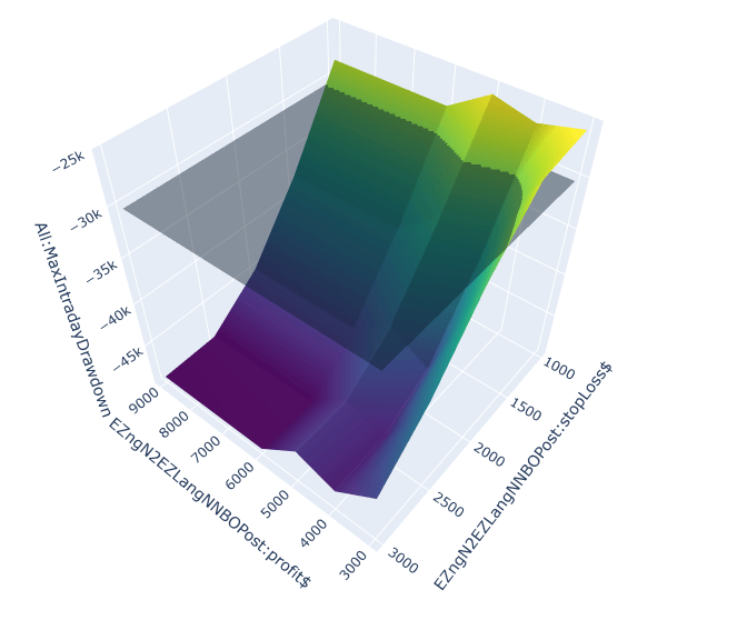
Risk.  Well, we are dealing with AI and Mag7 volatility here.  Very few results with less than a $30K draw down.  We are bumping up against the wall risking $1000 per trade.  We could push through the wall but I personally don’ think it is worth the effort.

Optimzation 2:

Objective function:  Net Profit

Plotting two parameters on a 3D chart is straightforward. Adding a third requires an extra step. We can still plot a result at each X–Y coordinate, but multiple results may now share that same coordinate because of the third parameter. To create one surface, we accumulate those results and plot their average at each unique X–Y location.

Reward.  Nice results across a nice high and level plateau, again.  The introduction of the Break-Even optimization changed the surface.  Remember we are looking at aggregate statistic at each X and Y not just one point.

Objective Function:  Maximum Draw down

Risk.  This was somewhat surprising.  The Break-Even addition returned all values (when averaged) at each X and Y between -$20K and -$30K.

Heat Map of Risk (3 parameters).  A chart like this is hard to see unless you rotate them.  I like to look at a Heat Map as well.  The following map shows a lower draw down values at lower stop loss and profit objectives.  Logical, right?

Heat Map of Risk (2 parameters).  What does the 2 parameter optimization heat map look like?

I think we can conclude the application of a Break-Even trade as a plus for the system.  Very few X and Y show desirable results.

Trade Filtering – Good or Bad:  Neither NR4 or NR7 were productive.  However, comparing yesterday’s True Range with the ATR produced some surprising results.

This demonstrates we need volatility but not too much volatility.  Trade filtering goes hand in hand with the amount you want to risk.  Filtering trades diminishes executions and therefore reduces exposure.

Final System:

Risk: $2000 – Reward: $9000 – BreakEven: $1500 – Volatility TR < 1.5 X ATR

Walk It Forward

Walked forward from August 2023 – this was the endpoint we used in the optimization process. A good fellow with just a hint of a temper.

Too much money too quickly!

Incubation Assessment
Overall Assessment: Degraded
Risk Assessment: High Risk
Incubation Readiness Score: 4 / 8
Return delivery is running ahead of baseline: expected annual return is 318% versus actual annual return of 434%, and expected annual gain of $39,732 compares with actual annual gain of $54,197. However, that stronger return delivery has come with a less stable path and/or materially heavier risk than history would suggest. Risk is materially worse than the historical profile: actual worst drawdown of $35,005 is 1.720 times the historical drawdown of $20,355. Risk conditions are in the High Risk range. The realized monthly path is no longer tightly aligned with the baseline, based on monthly equity correlation of 0.960, projection RMSE of $55,147, normalized RMSE of 1.388, and path wander ratio of 0.476.

Correlation still shows directional similarity, but the path wander ratio indicates noticeable drift away from the projected path over the same window. Monte Carlo context is cautionary: actual forward equity is $162,590, gain percentile is 78% (in the upper quartile), and drawdown percentile is 84% (in the upper quartile for drawdown stress). Taken together, the system shows meaningful deterioration in incubation.

That flat period at the beginning of the test period looks a little suspect, right?

Monte Carlo It

Running 2500 simulations with $50K initial capital and then extracting a typical year out of the results you get this:

This is what you get when you perform a Monte Carlo analysis over a time period that shows exceptional results.  However, the very best and very worst trades were removed first before the shuffling.

Top left corner is most dense quadrant = GOOD!

Walk it Backward!  Bell Bottom Jeans!

The 30-minute rule during this period of time was dismal.  Just like Bell Bottom jeans in the 1980s.

Generated Code Is Not the Same as Engineered Code

AI can write structure, but experienced programmers still supply the craft

The more we rely on generated code, the more disciplined we must become in questioning it.

AI and modern frameworks now provide valuable insights that, just a few years ago, would have required significant time and effort to obtain. However, while they offer tremendous macro-level leverage, they can also introduce subtle assumptions that lead to impossible scenarios and misleading downstream analysis. This is especially true in environments designed for rapid idea testing, where convenience can come at the expense of deeper, microscopic introspection.

For example, in my PatternSmasher framework, I use constructs like BarsSinceEntry to control trade duration and evaluate pattern efficacy. This makes it very easy to test thousands of ideas quickly. But that convenience comes with a responsibility. If you rely on these abstractions without thinking through the details, you can end up with behavior that looks perfectly valid in code but could never occur in the real world.

I have seen this problem in other frameworks and in AI-generated code as well. This is why it is so important to continue to hone your craft and take a deep dive into the results produced by generated code. In the quant world, the first step is to study the trades and isolate problems such as what I call simultaneous same-direction exit and reentry. Once you see it, the job is to fix it without changing the intent of the algorithm.

Let me show you exactly what I mean. The logic behind this example looks perfectly fine on the surface. But when you dig into the trades, you see the problem immediately. In this chart, the system exits a long position and then turns right around and buys again at the same time and price. That is not a reversal. It is a same direction exit and reentry that simply cannot happen in the real world, and it pollutes the back test with trades that should not exist.

Example of simultaneous same-direction exit and reentry at the same time and price—an impossible trade sequence that distorts backtest results – 640 minute bar on Gold – why 640?

We entered a long position, the trade expired, immediately re-entered on the next setup, that trade expired as well, and then entered again—only to get stopped out. That’s three round turns, each incurring commission and slippage.

// Simple code that is of course mean reversion.
// However, since we seem to be in this regime
// let's hone our craft to make this work as intended.

input:movAvgLen(50),consCloses(1),exitAfterNBars(5),stopLoss(3000);

value1 = countIF(c < c[1],consCloses);
value2 = countIF(c > c[1],consCloses);


if value1 = consCloses and close > average(c,movAvgLen) then
buy ("lentry") next bar at open;
if value2 = consCloses and close < average(c,movAvgLen) then
sellShort ("sentry") next bar at open;


if barsSinceEntry > exitAfterNBars then
Begin
sell("lx-exp") next bar at open;
buyToCover("sx-exp") next bar at open;
end;
setStopLoss(stopLoss);
Simple entry with expiration exit

The code that produced this looks pretty clean. You have your entry logic, a BarsSinceEntry exit, and a stop loss. On the surface, everything seems fine.

But you don’t find this kind of problem by staring at the code. You find it by looking at the trades.  This is the one thing AI or a framework doesn’t examine.  At first, the natural reaction is to slap a MarketPosition “gate” on the entry logic. The word “gate” may be a dead giveaway that AI has influenced the discussion. But I like it. It has been around since the early days of electrical circuits, and it is very appropriate here.  I’ve noticed that many of the words AI uses have started to creep into my own vocabulary. Funny how that happens.

Fix #1

input:movAvgLen(50),consCloses(1),exitAfterNBars(5),stopLoss(3000);

value1 = countIF(c < c[1],consCloses);
value2 = countIF(c > c[1],consCloses);


if marketPosition <> 1 and
value1 = consCloses and close > average(c,movAvgLen) then
buy ("lentry") next bar at open;

if marketPosition <> -1 and
value2 = consCloses and close < average(c,movAvgLen) then
sellShort ("sentry") next bar at open;


if barsSinceEntry > exitAfterNBars then
Begin
sell("lx-exp") next bar at open;
buyToCover("sx-exp") next bar at open;
end;
setStopLoss(stopLoss);
Fix #1 - solves the simultaneous exit and re-entry same direction glitch

So what does that MarketPosition “gate” actually do?

It fixes the symptom. The same-bar exit and reentry disappears, and the trades look cleaner.

But it also changes the algorithm in a much deeper way.

In the original design, a new long signal while already long reaffirmed the position and should have kept the trade alive. The gate removes that behavior. Now the strategy must exit first and then wait until the next bar to reenter.

And that delay matters.

By the time the next bar arrives, the setup may be gone. What should have been one continuous trade is now split into pieces—or missed entirely.

You didn’t just clean up the trades. You changed which trades exist.  The new strategy more or may not be more efficient, but just know the algorithm is now different.

Fix #2

We bought, suppressed the expiration exit due to a new buy setup—twice—and were ultimately stopped out at the level where the stop loss from the final trade that didn’t occur—but whose properties we were monitoring—would have been triggered.

Could most quants who aren’t programmers solve this riddle? Probably not. My 40 years of programming experience certainly played a role, and my familiarity with EasyLanguage—especially its limitations—helped guide me down the right path. But more importantly, I was able to recognize the nature of the problem, apply targeted fixes, and then analyze the resulting trades. I repeated this process—wash, rinse, repeat—until the issue was resolved.

Much of the knowledge I relied on has been documented by myself and others over the years. Investing time in books, videos, and webcasts specific to your programming language remains essential—it forms the foundation. But ultimately, refining your own skills and developing your craft is a time-consuming process that pays lasting dividends.

Groundwork for the Fix

Solving what initially appears to be a simple riddle requires recognizing several underlying behaviors. I was able to correct the issue because I could anticipate when a new trade was about to occur. When both the exit gate for an existing position and the entry gate for a new position in the same direction were simultaneously open, I prevented the transition by closing both gates.

However, simply blocking the transition was not enough. I had to simulate the trade that would have occurred. This meant marking the hypothetical entry price, resetting the stop-loss based on that price, and reinitializing my own bars-in-trade counter.

At this point, I could no longer rely on EasyLanguage’s built-in functions such as BarsSinceEntry or SetStopLoss. Those functions assume an actual executed trade and therefore could not reflect the internal state I needed to maintain. To solve the problem correctly, I had to take full control of trade state management and explicitly track these values myself.

input:movAvgLen(50),consCloses(1),exitAfterNBars(5),stopLoss(3000);

vars: mp(0),barsMult(1),barsIntrade(0),lStopLevel(0),sStopLevel(0),closedTrades(0);
vars: canGoLong(False),canGoShort(False);

canGoLong = countIF(c < c[1],consCloses) = consCloses and close > average(c,movAvgLen) ;
canGoShort = countIF(c > c[1],consCloses) = consCloses and close < average(c,movAvgLen);

mp = marketPosition;

//Exit Technology

closedTrades = totalTrades;
//long exit on bar after entry
if mp[1] <> mp and mp = 1 or (closedTrades > closedTrades[1]) Then
begin
barsInTrade = 0;
lStopLevel = open[0] - stopLoss/bigPointValue ;
end;

//short exit on bar after entry
if mp[1] <> mp and mp = -1 or (closedTrades > closedTrades[1]) Then
begin
barsInTrade = 0;
sStopLevel = open[0] + stopLoss/bigPointValue ;
end;

//long reentry stop reset
if mp = 1 and canGoLong and barsInTrade > exitAfterNBars Then
begin
lStopLevel = open of tomorrow - stopLoss/bigPointValue ;
// print(d," ",t," should exit and renter long tomorrow ",barsInTrade," ",barsSinceEntry," ",open of tomorrow);
barsInTrade = -1;
end;

//short reentry stop reset
if mp = -1 and canGoShort and barsInTrade > exitAfterNBars Then
begin
sStopLevel = open of tomorrow + stopLoss/bigPointValue ;
// print(d," ",t," should exit and renter short tomrorrow ",barsInTrade," ",barsSinceEntry," ",open of tomorrow);
barsInTrade = -1;
end;

if mp = 1 then
sell("lx-stopLoss") next bar at lStopLevel stop;

if mp = -1 then
buyToCover("sx-stopLoss") next bar at sStopLevel stop;

//Entry Logic
if canGoLong then
buy ("lentry") next bar at open;
if canGoShort then
sellShort ("sentry") next bar at open;


//Bars in trade expiration exit
if barsInTrade > exitAfterNBars then
Begin
sell("lx-exp") next bar at open;
buyToCover("sx-exp") next bar at open;
end;

//Day of entry protection
setStopLoss(stopLoss);
//Increment barsInTrade - mimic TradeStation here too!
if mp <> 0 then barsInTrade = barsInTrade + 1;
Fix #2 - difficult initially but reusable

This version fixes the problem by taking control of the trade state instead of relying on EasyLanguage’s built-in functions.

First, I define whether I can go long or short, independent of my current position. Then I track my own state variables—market position, bars in trade, stop levels, and trade count—so I know exactly what the system is doing at all times.

The key occurs when a same-direction signal appears after the trade has technically expired. Instead of allowing an exit and immediate reentry, I suppress both actions and simulate the renewed trade. I mark the hypothetical entry price, reset the stop based on that level, and restart my bars-in-trade counter.

Because of this, I can no longer rely on BarsSinceEntry or SetStopLoss—they depend on actual trades. I manage everything explicitly.

The result is a continuous position that preserves the original intent of the algorithm without introducing impossible trades into the backtest.

EasyLanguage also has its share of esoteric nuances. Code order can matter in some places and not in others, particularly with order execution. Even detecting position changes requires a bit of finesse. These details matter, but they are beyond the scope of this discussion.

This is where the difference between generated code and engineered code becomes clear.

A programmer who is not willing to put in the work—and instead relies on AI to solve the problem—will likely stop at the first acceptable fix. The code will run, the trades will look cleaner, and the issue will appear resolved. But the deeper problem remains: the structure has changed, trades may be missing, and the original intent of the algorithm has been compromised.

As we become more dependent on code generation through AI and frameworks, it becomes even more important to validate that the output is reasonable and reflects something that could occur in the real world. That responsibility does not go away—it increases. And it requires us to continue honing our craft.

AI can generate code and even suggest reasonable fixes, but it does not truly understand the nuances of the language, the sequencing of events, or the intent behind the strategy. It cannot look at a trade and say, “that shouldn’t have happened.” It does not debug by questioning reality—it follows patterns.

Arriving at the correct solution required recognizing the problem, iterating through possible fixes, examining the trades, and refining the logic until the behavior matched the intent. That process—wash, rinse, repeat—is the craft.

Generated code can get you started. Engineered code is what gets you to the truth.  Take a look at the two following reports.  Similar results, but look at the number of trades and those statistics tied to this number.


A Turtle Thermometer for Trend-Following: 2025 Results

A Bare-Bones Turtle Algorithm for Gauging Trend-Following Conditions

The core Turtle rules were fully mechanical, but several operational choices, such as position sizing nuances, market selection, roll/contract handling, and execution practices were left to judgment or circumstance. Many would argue the philosophy behind the Turtles mattered as much as the rules themselves, and differing interpretations of that philosophy go a long way toward explaining why their results diverged so widely. The mechanics, however, are straightforward: you can distill them from the published books and courses, strip them down even further, and apply the resulting rule set across a broad portfolio to take the pulse of trend-following today.

I’ve worked with the Turtle framework for many years, coded numerous variants, and even compared notes with a handful of original Turtles. If any method can “take the temperature” of market trendiness, this one can. This system synthesizes a shorter-term trend mechanism (that limits execution based on the prior outcome) with a true longer term trend following entry and exit method (two months of data are used to determine entry).   Short-term trading is difficult and often falls victim to over trading.  The shorter-term entry is used to try and capitalize on the genesis of a big trend.  Preventing another trade after a winner is one method of reducing trading and chop.  If the short-term break out turns into a trend and entry is prevented, then the 55-day break out is there to capture it.  Below are the rules I extracted to build a fully mechanical, bare-bones algorithm for that purpose.

Rules Used in This Analysis

Conventions & Definitions

  • Breakout (stop basis): Enter on a stop when price exceeds the specified lookback extreme by 1 tick (or exactly at the extreme if your platform supports that).
  • N: 20-day weighted Average True Range (WATR) used for both systems.
  • Risk stop (volatility stop): A stop placed 2×N from the entry price.
  • Swing stop: For System #1, use the 10-day highest high/lowest low; for System #2, use the 20-day highest high/lowest low.
  • Closest stop wins: The active protective stop at any time is the tighter of the risk stop and the swing stop.
  • Loser vs. non-loser (for System #1’s gating rule):
    • A trade that is stopped out by 2×N is a loser.
    • A trade that exits via the 10-day swing stop (even if it’s a loss) is not counted as a loser for gating.
    • Profitable exits via the 10-day swing stop are obviously not losers.

System #1 — 20-Day Breakout (Conditional)

Purpose: Only take the next 20-day breakout if the most recent 20-day breakout resulted in a 2×N loss.

  • Entry condition (gated):
    • Compute the 20-day Donchian channel.
    • You may only take a long (new 20-day high) or short (new 20-day low) breakout if the last System #1 trade ended with a 2×N risk stop.
    • If the last System #1 trade exited via the 10-day swing stop, it does not unlock the gate.
  • Initial protective stops (at entry):
    • Risk stop: 2×N from entry.
    • Swing stop: Opposite extreme of the past 10 days (lowest low for longs, highest high for shorts).
    • Use the tighter of the two stops at all times (“closest stop wins”).
  • Exit rules:
    • Exit if price hits the active stop (risk or swing).
  • Bookkeeping for gating:
    • If exit was the 2×N risk stop, mark the trade as a loser (this unlocks the gate for the next entry).
    • If exit was the 10-day swing stop, do not mark as a loser (gate remains locked).
  • Always evaluating: System #1’s breakout logic runs continuously, but entries are allowed only when the gate is unlocked by a prior 2×N loss.


System #2 — 55-Day Breakout (Always On)

Purpose: Classic trend capture that runs regardless of System #1’s state; does not affect System #1’s gating.

  • Entry condition (ungated):
    • Enter long on a 55-day high breakout; enter short on a 55-day low breakout.
  • Initial protective stops (at entry):
    • Risk stop: 2×N from entry.
    • Swing stop: Opposite extreme of the past 20 days (lowest low for longs, highest high for shorts).
    • Use the tighter of the two stops at all times.
  • Exit rules:
    • Exit if price hits the active stop (risk or swing).
  • Isolation from System #1:
    • System #2 trades and outcomes do not influence System #1’s “last-trade-was-a-loser” gate (also known as a filter).

The Portfolio

Currencies (CME FX)

Preferred name Short Futures ticker
Australian Dollar AUD @AD (6A)
British Pound GBP @BP (6B)
Canadian Dollar CAD @CD (6C)
Euro EUR @EC (6E)
Japanese Yen JPY @JY (6J)
Swiss Franc CHF @SF (6S)

Rates (CBOT)

Preferred name Short Futures ticker
30-Year U.S. Treasury Bond 30Y @US (ZB)
10-Year U.S. Treasury Note 10Y @TY (ZN)
5-Year U.S. Treasury Note 5Y @FV (ZF)

Equity/Index

Preferred name Short Futures ticker
E-mini S&P 500 ES @ES (CME)
U.S. Dollar Index DXY @DX (ICE)

Metals (COMEX/NYMEX)

Preferred name Short Futures ticker
Gold XAU @GC
Copper Cu @HG
Silver XAG @SI
Palladium Pd @PA=11INC
Platinum Pt @PL

Energies (NYMEX)

Preferred name Short Futures ticker
RBOB Gasoline RBOB @RB
Heating Oil HO @HO
WTI Crude Oil WTI @CL
Henry Hub Natural Gas NatGas @NG

Grains/Oilseeds (CBOT)

Preferred name Short Futures ticker
Soybeans Beans @ZS
Corn Corn @ZC
Rough Rice Rice @ZR
Wheat (SRW) Wheat @ZW
Soybean Meal Meal @ZM

Livestock (CME)

Preferred name Short Futures ticker
Feeder Cattle Feeders @FC (GF )
Live Cattle LiveCat @LC (LE )
Lean Hogs Hogs @LH (HE)

Softs (ICE)

Preferred name Short Futures ticker
Frozen Concentrated Orange Juice OJ @OJ
Sugar No. 11 Sugar @SB
Cotton No. 2 Cotton @CT
Coffee “C” Coffee @KC
Lumber Lumber @LBR = @LB legacy

Market Normalization (Fixed-Fractional Sizing)

To level the playing field across markets, I used fixed-fractional position sizing keyed to the Turtle “quick” 20-day ATR.

Risk budget per trade

  • Account equity =$250,000
  • Fraction at risk per trade =2%
  • Dollar risk per trade: = × = 0.02 × 250,000 = $5,000

Contracts to trade

  • Let ATR = 20-day (Turtle quick) Average True Range in price units
  • Let BPV = Big Point Value (dollars per 1.0 move)
  • Dollar risk per 1 contract: ATR × BPV
  • Position size (contracts):
  • Contracts =⌊ / ATR × BPV⌋

In words: allocate $5,000 of risk to each trade and size the position by dividing that risk by the market’s expected dollar move (ATR×BPV).   Round down to an integer.

Notes & conventions
  • ATR is the 20-day Turtle quick ATR (same used in the rules).
  • Use the correct BPV for each contract (e.g., ES $50/pt, CL $1,000/pt, SI $5,000/pt).
  • Enforce at least on contract per signal.
  • $50 slippage and $10 commission per round turn.

Results

Large portfolio performance on Bare Bones Turtle

This equity curve is very typical across the spectrum of most trend following systems.  There have been big years to keep the trend following momentum going – recently 2008, 2010, 2014, 2018, 2020.

Big Years – pushes the popularity of Trend Following

Many times, the futures and commodity markets are there to benefit from global events such as the banking collapse (2008) and the pandemic (2020).

Over the years, markets have fallen in and out of favor with Trend Following.  The best market over the past twenty years or so turned out to be sugar.  With its smaller size and associated volatility and trends it was the clear winner.

Many HOT SPOTS on the Correlation Heat Map

Pearson Correlation Matrix

But, what about smaller accounts?

There exist sub portfolios with better profit to draw down ratios.  If you could only choose ten markets and wanted to know the best combination, you can do this with my TS-PortfolioMerge software.  In fact, all the metrics and images I have shown in this post were generated with TS-PortfolioMerge.  If your budget only allows for 10 markets and you want to evaluate every combination you will need to wait a while for TS-PM to run through every combination.

Search space C(37,10) = 348,330,136 (subset) – yes that is 300 million combinations.  Just set up your computer for overnight processing.

But if you want a speedy answer, that will approximate the entire search space you can do that as well.

Sampled (limit 50,000; randomized).

# P/DD Net Profit ($) Max DD ($) Symbols
1 12.071 1,615,758.97 133,857.91 @EC, @HG, @HO, @JY, @LB=11INC, @LH, @RB, @SB, @SM, @TY
2 11.676 1,333,359.10 114,194.85 @FC, @GC, @HO, @KC, @LB=11INC, @LBR=11INC, @LH, @OJ, @SB, @SM
3 11.563 1,473,201.00 127,410.20 @C, @CL, @EC, @ES, @GC, @HG, @HO, @LBR=11INC, @LH, @SB
4 11.545 1,601,806.50 138,745.50 @C, @CL, @CT, @GC, @HO, @LH, @RB, @SB, @SM, @US
5 11.444 1,427,082.85 124,705.40 @CL, @GC, @HO, @KC, @LB=11INC, @LBR=11INC, @LH, @OJ, @S, @SB

Run the speedy version multiple times to see if the same portfolio bubbles to the top.  If you continue getting different portfolios, you can run the exhaustive mode.  Here the best 10 markets were:

@EC, @HG, @HO, @JY, @LB=11INC, @LH, @RB, @SB, @SM, @TY

Here you have two currencies (EC and JY), one metal (HG), two energies (HO and RBOB), one interest rate (TY), sugar, lumber, soybean meal and lean hogs.  But are we guilty of cherry picking?  Maybe the Monte Carlo analysis will provide some insight.

Monte Carlo Analysis on 10 of the best combination from the Speedy output.

Conclusion

Trend Following as of late October 2025 is doing well and doing as expected.  The pandemic pulled the algorithm out of the doldrums and positive years have been banked since.  The current year looks like the exception, but we still have two months left.  With the Gold move you would think 2025 would have been a banner year.  The Trend is STILL OUR FRIEND.

Email me if you would like my code for my bare bones Turtle system, I utilized to create all these results.  The code includes the human curated LAST TRADE WAS A LOSER function.

Can the Recursive Gaussian Channel Beat the Battle Tested Bollinger Band?

Bridging 19th‑century mathematics and 21st‑century trading methods

A client sent me what looked like a simple indicator written in TradingView’s Pine Script—though I didn’t realize it was Pine at first—and asked if I could port it to EasyLanguage (or PowerLanguage for MultiCharts). If you Google “Gaussian Channel Donovan Wall TradingView,” you’ll find the original code. Pine Script isn’t exactly newcomer-friendly; it’s fine once you get the feel for it, but I’m spoiled by EasyLanguage, which —at least to my eye—reads almost like plain English. (Others may beg to differ!) Below is a brief Pine snippet; to this humble EL devotee, it’s more hieroglyphics than prose.

    _m2 := _i == 9 ? 36  : _i == 8 ? 28 : _i == 7 ? 21 : _i == 6 ? 15 : _i == 5 ? 10 : _i == 4 ? 6 : _i == 3 ? 3 : _i == 2 ? 1 : 0
_m3 := _i == 9 ? 84 : _i == 8 ? 56 : _i == 7 ? 35 : _i == 6 ? 20 : _i == 5 ? 10 : _i == 4 ? 4 : _i == 3 ? 1 : 0
_m4 := _i == 9 ? 126 : _i == 8 ? 70 : _i == 7 ? 35 : _i == 6 ? 15 : _i == 5 ? 5 : _i == 4 ? 1 : 0
_m5 := _i == 9 ? 126 : _i == 8 ? 56 : _i == 7 ? 21 : _i == 6 ? 6 : _i == 5 ? 1 : 0
_m6 := _i == 9 ? 84 : _i == 8 ? 28 : _i == 7 ? 7 : _i == 6 ? 1 : 0
_m7 := _i == 9 ? 36 : _i == 8 ? 8 : _i == 7 ? 1 : 0
_m8 := _i == 9 ? 9 : _i == 8 ? 1 : 0
_m9 := _i == 9 ? 1 : 0

I could see right away that the code was doing some kind of coefficient “lookup,” so I ran it through ChatGPT to get a quick explanation. The model suggested it was building weights from Pascal’s Triangle. A bit later the client sent me the original TradingView post, which confirmed the script was using John Ehlers’s Gaussian filter to build a channel—similar in spirit to Keltner or Bollinger bands.

Once Ehlers’s name popped up, the next stop was his resource-rich site (mesasoftware.com/TechnicalArticles) for the theory behind the filter. I also searched for a ready-made EasyLanguage version but came up empty. With ChatGPT’s help I decided to roll my own; after all, knocking out support code like this is exactly what these AI tools are for.

What do Carl Friedrich Gauss, Blaise Pascal, and the markets have in common.

You’ve probably bumped into the bell curve in school—maybe in a stats class, maybe when teachers “graded on a curve.” Mathematicians call it by a few interchangeable names:

  • Normal distribution (stats class)
  • Gaussian curve (named after Carl Friedrich Gauss)
  • Binomial curve (because it pops out of Pascal’s Triangle)

No matter the label, it’s the same smooth hump that says, “most values cluster in the middle, very few at the extremes.” Gauss formalized the formula, Pascal’s Triangle supplies the ready‑made integer weights, and traders borrow both ideas to build filters that tame noisy price charts.

Big picture: Gauss gives us the shape of the curve, Pascal gives us the exact numbers to approximate it, and that combo lets us create a market indicator that reacts quickly and stays smooth.

How does this help build an indicator?

The word channel is in the name of the indicator, so it was highly likely we are dealing with a smoothed price with an upper and lower band a certain distance from the smoothed price.  If you feed this into Chat GPT and ask for it in EasyLanguage, it will create an indicator using a bunch of arrays.  See Chat GPT isn’t 100% knowledgeable of EasyLanguage like it is with python.  It didn’t understand the concept of EasyLanguage’s serialized variables.  You know where you can refer to a prior value of a variable – myValue[1] or myValue[2].  Chat tries to replicate this with the usage of arrays which gets you into a bunch of trouble right off the bat.  Let’s discuss this a little later.

The Mechanics of smoothing price with Pascal’s Triangle, or Gaussian Kernal or Binomial Coefficients.

(a + b)^2 = a^2 + 2ab + b^2 → coefficients 1  2  1

(a + b)^3 = a^3 + 3a^2b + 3ab^2 + b^3 → coefficients 1 3 3 1

(a + b)^4 = a^4 + 4a^3b + 6a^2b^2 + 4ab^3 + b^4 → coefficients 1 4 6 4 1

(a + b)^5 → coefficients 1 5 10 10 5 1

(a + b)^6 → coefficients 1 6 15 20 15 6 1

(a + b)^7 → coefficients 1 7 21 35 35 21 7 1

(a + b)^8 → coefficients 1 8 28 56 70 56 28 8 1

(a + b)^9 → coefficients 1 9 36 84 126 126 84 36 9 1
Binomial Coefficients

Stack those rows, keep going, and you build Pascal’s Triangle—each number is the sum of the two numbers just above it.

Look at the 7th row of Pascal’s Triangle:

1  6  15  20  15  6  1

Normalize those numbers (divide by their sum), and you obtain a discrete approximation of a Gaussian kernel.  Big Deal, right?  You don’t need to know the math behind this, just know that each row in Pascal’s triangle is symmetric.  Each row starts are one and ends at one.  You can use these coefficients to weight each value across a period of time.  Do you mean all this math stuff is akin to a weighted moving average.

Idea Weighted Moving Average Binomial / Gaussian weights Why they feel similar
What it does Averages recent prices, but gives newer bars bigger weights (e.g., 1-2-3-4). Averages recent prices using the numbers from Pascal’s Triangle (e.g., 1-4-6-4-1). Both are just weighted sums of past prices.
Shape of the weights Forms a triangle – rises steadily to the newest bar, then drops to zero beyond the window. Forms a bell – climbs to the centre, then falls off symmetrically. Triangles and bells are both peaked shapes: the middle matters most, the edges least.
Normalizing step Divide by the sum of the weights (e.g., 1+2+3+4 = 10) so they add to 1. Same: divide by 1+4+6+4+1 = 16 so they add to 1. After normalizing, each is just a fancy way to say “take a percentage of each bar and add them up.”
Smoothing power Good at knocking out single-bar noise, but the straight sides of the triangle let more mid-frequency wiggles through. Slightly better at suppressing both very fast and mid-speed wiggles, so the line looks cleaner. Both cut random jitter while trying not to lag too far behind real turns.
Math connection A single pass of linear weights. What you get if you apply a two-point moving average over and over again (each pass builds the next Pascal row). Re-applying a simple WMA repeatedly evolves into the binomial weights – that’s the family link.

Which comes first the indicator or the function that feeds the indicator?

If you are working with code and especially with ChatGPT or any other LLM you need a medium where you can quickly program and observe results.  The indicator analysis module will give you instant results. and this is where you should start.  However, if you look at the TradingView code of the Gaussian Channel you will notice that the smoothing function is called twice, once for the close and once for the true range on each bar.  In other words, you are using the same code twice and incorporating this without functions would be redundant.  In my first attempt, I created the smoothing function and named it Binomial, and the channels were a magnitude of 10 below the current price.  So, all the price bars were scrunched at the very top of the chart.  At first if you don’t succeed, try and try and try and try again.

At first ChatGPT kept insisting on arrays because it didn’t realize EasyLanguage can reference earlier bars just by tagging a variable with [n]. EasyLanguage conveniently hides that bookkeeping, but you have to tell the model so it stops reinventing circular buffers. Once I explained that a local variable—say filt—already remembers its prior values (filt[1], filt[2], etc.), the conversation moved forward.

The next hurdle was clarifying that Donovan’s script feeds raw data (Close and TrueRange) into every stage, not the output of the previous stage. ChatGPT was trying to build a true cascade—each pole using the prior pole’s result—whereas Donovan calculates each pole completely independently. After I pointed that out, the model rewrote the logic correctly and even walked me through the difference:

  1. Cascaded filter → Pole 2 uses Pole 1’s output, Pole 3 uses Pole 2’s, and so on.

  2. Independent poles → Every pole starts over with the raw Close and Range.

That explanation finally squared the circle and let me produce an EasyLanguage version that matches the original TradingView indicator.

“Cascade” = one stage feeding the next

Think of a cascade as a relay race:

  1. Stage 1 (“Pole 1”) takes the raw price, smooths it a little, and hands the baton to …

  2. Stage 2 (“Pole 2”), which smooths the output of stage 1 a bit more, then passes to …

  3. Stage 3, and so on.

After 4-, 6-, or 9-hand-offs the combined shape of all those little smooths matches the full Gaussian bell.


The indicator lets you pick anywhere from two to nine poles to do the heavy lifting on the data-smoothing. And no, we’re not talking about the North and South Poles—or the kind you cast a fishing line from.

So, what is a pole?

In filter speak, a pole is one little “memory stage” inside the math that reaches back to yesterday’s value (or last bar’s value) before deciding today’s output. Stack more poles and you stack more of those memory stages:

  • 1 pole → basically a quick-and-dirty exponential average.

  • 4 poles → four mini-averages chained together; much smoother, a hair more lag.

  • 9 poles → nine stages deep; super-silky curve, but you’ll feel the delay.

Think of each pole as a coffee filter. One filter catches the big grounds, two filters catch the sludge, and by the time you’ve got nine stacked up, you’re practically drinking distilled water. Same beans in, different smoothness out.

You can dial in two extra tweaks:

  • Lag compensation – Tell the code to look one step ahead by swapping in a one-bar forecast of price for the raw price. That little nudge pulls the channel forward so it doesn’t trail the market.
  • Extra smoothing – Want the line even silkier? Flip the switch and the function just averages the most-recent two filter values. It’s a tiny moving average—jitter drops a notch, lag creeps up by only half a bar.

For illustrative purposes this is how Pole 6 is calculated.  I also show a mapping scheme to store Pascal’s triangle into arrays.  I put all this code inside a function with the name BinomialFilterN.

{─────────────────────────────────────────────────────────────────────
2. Hard-code every Pascal row (n = 1 … 9)
─────────────────────────────────────────────────────────────────────}
once
begin
{ n = 1 : 1 1 }
m0Map[1] = 1; m1Map[1] = 1;

{ n = 2 : 1 2 1 }
m0Map[2] = 1; m1Map[2] = 2; m2Map[2] = 1;

{ n = 3 : 1 3 3 1 }
m0Map[3] = 1; m1Map[3] = 3; m2Map[3] = 3; m3Map[3] = 1;

{ n = 4 : 1 4 6 4 1 }
m0Map[4] = 1; m1Map[4] = 4; m2Map[4] = 6; m3Map[4] = 4;
m4Map[4] = 1;

{ n = 5 : 1 5 10 10 5 1 }
m0Map[5] = 1; m1Map[5] = 5; m2Map[5] = 10; m3Map[5] = 10;
m4Map[5] = 5; m5Map[5] = 1;

{ n = 6 : 1 6 15 20 15 6 1 }
m0Map[6] = 1; m1Map[6] = 6; m2Map[6] = 15; m3Map[6] = 20;
m4Map[6] = 15; m5Map[6] = 6; m6Map[6] = 1;

{ n = 7 : 1 7 21 35 35 21 7 1 }
m0Map[7] = 1; m1Map[7] = 7; m2Map[7] = 21; m3Map[7] = 35;
m4Map[7] = 35; m5Map[7] = 21; m6Map[7] = 7; m7Map[7] = 1;

{ n = 8 : 1 8 28 56 70 56 28 8 1 }
m0Map[8] = 1; m1Map[8] = 8; m2Map[8] = 28; m3Map[8] = 56;
m4Map[8] = 70; m5Map[8] = 56; m6Map[8] = 28; m7Map[8] = 8;
m8Map[8] = 1;

{ n = 9 : 1 9 36 84 126 126 84 36 9 1 }
m0Map[9] = 1; m1Map[9] = 9; m2Map[9] = 36; m3Map[9] = 84;
m4Map[9] = 126; m5Map[9] = 126; m6Map[9] = 84; m7Map[9] = 36;
m8Map[9] = 9; m9Map[9] = 1;
end;

{─────────────────────────────────────────────────────────────────────
3. Working variables
─────────────────────────────────────────────────────────────────────}
variables:
beta_(0), { = 1 – alpha }
f1(0), f2(0), f3(0), f4(0), f5(0),
f6(0), f7(0), f8(0), f9(0),
f(0);

beta_ = 1 - alpha;

{─────────────────────────────────────────────────────────────────────
4. Initialise memory until we have enough bars
─────────────────────────────────────────────────────────────────────}
if currentBar <= poleCount then
begin
f1 = 0; f2 = 0; f3 = 0; f4 = 0; f5 = 0;
f6 = 0; f7 = 0; f8 = 0; f9 = 0;
end
else
begin
{================== 1-pole ==================}
if poleCount = 1 then
begin
f1 = m0Map[1]*power(alpha,1)*source
+ m1Map[1]*power(beta_,1)*f1[1];
f = f1;
end;

{================== 2-pole ==================}
{================== 3-pole ==================}
{================== 4-pole ==================}
{================== 5-pole ==================}
{================== 6-pole ==================}

if poleCount = 6 then
begin
f6 = m0Map[6]*power(alpha,6)*source
+ m1Map[6]*power(beta_,1)*f6[1]
- m2Map[6]*power(beta_,2)*f6[2]
+ m3Map[6]*power(beta_,3)*f6[3]
- m4Map[6]*power(beta_,4)*f6[4]
+ m5Map[6]*power(beta_,5)*f6[5]
- m6Map[6]*power(beta_,6)*f6[6];
f = f6;
end;
Code showing Pascal's Triangle and 6 pole smoothing

There is redundant code here, but I included it to make it readable for most of my EasyLanguage/PowerLanguage programmers.   The math is very simple when you break it down.  If we choose Pole #6 all we do is:

beta_ = (1 – Cosine(360 / per)) / (Power(1.414, 2 / numPoles) – 1);
alpha = -beta_ + SquareRoot(beta_ * beta_ + 2 * beta);

  1. 1 x alpha^6 x close
  2. plus 6 x beta^1 x prior f6[1]
  3. minus 15 x beta^2 x f6[2]
  4. plus 20 x beta^3 x f6[3]
  5. minus 15 x beta^4 x f6[4]
  6. plus 6 x beta^5 x f6[5]
  7. minus 1 x beta^6 x f6[6]

EasyLanguage’s trig calls expect degrees, while most other languages want radians. That’s why the code feeds Cosine(360 / per)—the 360 converts the cycle length into degrees before taking the cosine.

I also lift the constant √2 (1.414…) by squaring it with Power(1.414, 2)and use the same Power routine for roots—for example, the cube root of x is simply Power(x, 1 / 3).

I placed BinomialFilterN inside a second routine called GaussianChannelFunc—a classic wrapper.

Why bother with the extra layer?

Reason What the wrapper does before/after calling BinomialFilterN
Housekeeping • Converts the user-friendly period (per) into the α required by the core filter.• Optional one-bar “look-ahead” to cancel lag.• Runs the filter twice (price and TrueRange).
Packaging • Builds upper, centre, and lower bands from the two filtered series.• Returns all three numbers through one array argument.
Extensibility Tomorrow you can tweak the channel logic—different volatility measure, ATR multiplier, extra smoothing—without touching the filter math. The heavy-duty code stays in BinomialFilterN; the wrapper simply preps inputs and formats outputs.

Think of it as a coffee machine:

  • BinomialFilterN is the brewing unit—hot water + grounds in, espresso out, and it never changes.
  • GaussianChannelFunc is the barista: grinds the beans, measures the water, adds milk and foam, then hands you the finished latte. If you want vanilla syrup tomorrow, you ask the barista; you don’t redesign the boiler.

By splitting the work this way, each piece stays focused, easier to test, and simple to extend later.

The wrapper has to hand back three numbers—upper band, centre line, and lower band—yet an EasyLanguage function can formally return only one. The standard workaround is to pass the additional outputs by reference:

// upper are caught by the receiving function as type numericRef
// can get unweilding quickly
value1 = GaussianChannelFunc(src, periods, numOfPoles,compLag, smooth, upper, mid, lower);
Code Snippet - Calling the function with three containers for the levels

That works, but the call quickly turns into a mile-long argument list.
Instead, I bundle those three outputs into a tiny array and pass the array’s address once:


array:GaussianChanArray[3](0); // remember we can use [0]

value1 = GaussianChannelFunc(src, periods, numOfPoles, compLag, smooth,GaussianChanArray);

upperChannel = GaussianChanArray[0];
centreLine = GaussianChanArray[1];
lowerChannel = GaussianChanArray[2];
Using a simple array as container for return values

This wasn’t that impressive, but what if your function needed to return five values?

Now onto the indicator and the strategy

From the outside this looks like a quick coding job—but getting here was a series of detours. I let ChatGPT drive and only nudged when it went off-track. Here are the dead-ends we hit before the indicator finally behaved:

  • Pine-script blind spot
    • ChatGPT didn’t recognise TradingView syntax, so its first translation attempts were gibberish.
  • “Mystery math” instead of binomial weights
    • After I mentioned Ehlers and Gaussian smoothing, the model invented a dynamic weighting scheme rather than using the fixed Pascal-triangle numbers the original script relies on.
  • Arrays everywhere
    • It kept insisting on circular buffers because it didn’t realise EasyLanguage variables already remember their own history via [1], [2], etc.
  • Wrong memory reference
    • Even after the array issue was fixed, the code updated each pole with raw price / range instead of the pole’s own prior output.
  • Unwanted filter cascade
    • ChatGPT then tried a true “cascade” (pole 2 fed by pole 1, pole 3 by pole 2). Donovan’s version calculates every pole independently—so we had to unwind that and start over.
  • Sign-flip confusion
    • It forgot the plus/minus pattern that keeps the Gaussian zero-lagged, producing a line that trailed price by several bars.

Each course-correction tightened the spec until the model finally spit out the straight, hard-coded-coefficients version you see now.

After all that was it worth the time and analysis?

  • A stop version where you buy at and sell short at the upper and lower levels worked best.  Liquidating at the midlevel on a stop was also incorporated.
  • Using a large profit objective and a relatively small stop loss seemed to work best.
  • Intermediate period length and utilizing 8 poles produced the best results.

ELD for TradeStation and Multicharts

GAUSSIANSTUDY

Text files of functions, indicator and strategies

GaussianChannelFunc Function

Head to Head with Bollinger Bands

Test results across 22 commodities for the past 25 years.

Gaussian Channel:  Optimizing the period and ATR multiplier with 8 poles:

Simple Bollinger Band: optimizing moving average length and number of standard deviations

Conclusion (fight-card style)

Decision on the first bout:
The Rolling heavy-hitter—Bollinger Bands—lands the cleaner power shots and takes the scorecards in our 22-commodity test.

But don’t call it a knockout just yet.
The Recursive counter-puncher—the Gaussian Channel—fights with an extra weapon: pole count. Adjusting those poles changes how tightly the centre line hugs price, and we’ve only sparred with one setting.

Next round:
Tune the poles, test different time-frames, and pit the fighters on equities and FX. The smarter, jabbing Gaussian might steal the rematch once its footwork is dialed in.


Unlocking Sequential™ in EasyLanguage via Dueling Finite State Machines

Disclaimer:
“Sequential™” is a registered trademark of Tom Demark. This post presents an independent, educational interpretation of the components of the Sequential™ pattern as described in Tom Demark’s book, The New Science of Technical Analysis. The analysis, opinions, and code examples provided herein are solely those of the author and are intended for informational and educational purposes only. This work is not affiliated with, endorsed by, or officially connected to Tom Demark or any related entities.

Sequential™ Pattern – Setup and Countdown

This pattern is fully described in Tom Demark’s book and consists of two distinct phases.  For brevity’s sake, I will just discuss the buy setup.  This indicator is designed to help determine when a trend is becoming or has become exhausted.  Unlike a trend following indicator that helps you get in at the genesis of the trend, Sequential indicates when to take an opposing position after trend termination.  This post doesn’t concern itself with the efficacy of Sequential, but with the process of programming such a difficult pattern and all the conditions that it involves.  The indicator consists of two parts or phases. The Setup phase is stringent, requiring that the same price pattern occur for at least nine consecutive days (bars). In contrast, the Countdown phase is less strict; it mandates that a different price pattern occurs over a span of 13 days (or bars), although these occurrences do not need to be consecutive.  Setup is complete when an “intersection” occurs, marking the point where prices start to brake or consolidate. Countdown, on the other hand, is finished when the 13th instance of the designated price pattern is observed. Because the pattern in the Countdown phase does not have to appear on consecutive bars, this phase can take many days to complete.  During Countdown, three scenarios can occur that either restarts or recycles the process.

Setup – Sequence

  1. close[0] > close[4]
  2. followed by nine consecutive Close[0] < Close[4]

Intersection- Sequence

  • If nine bars fulfill the Setup then examine the following
    • Bar 8  High[1] > Lowest(Low[4],5)
    • Bar 9  High[0] > Lowest(Low[3],5)

Countdown – Sequence

  • 13 days or bars fulfill Close[0] < Low[2] over any number of days

Sequential™ – Completion, Restart, Recycle

  • Completion – once Countdown reaches 13, the Sequential pattern is completed.
  • Restart – during countdown if a Close > Highest High during setup or a Sell Setup occurs – start either from scratch or start the Sell Countdown
  • Recycle – a new Buy Setup occurs, then start from the Countdown phase again.

Because we have to monitor a Sell Setup during the Countdown phase, we need to run two Finite State Machines concurrently.  These two state machines will duel with each other.  Both searching for their own solutions and knocking each other out during the process.

Finite State Machine Structure

Years ago, I embarked on building a theoretical compiler—a challenging project I nearly finished. The initial step was to create a parser that transforms high-level code into tokens according to the language’s grammar. In doing so, I learned about Finite State Machines (FSMs) as my program processed source code one character at a time and used FSM logic to build a token table.

Sample FSM to Find Pivot Highs and Pivot Lows

From this experience, I quickly discovered that even the most complex patterns can be detected using a Finite State Machine. Below is a graphical representation of a simple FSM that identifies the following pattern that can take up to 90 days (bars) to complete.

  1. A high pivot with strength 2

  2. Followed by a low pivot with strength 2

  3. Followed by another high pivot with strength 2

In this example, a pivot is defined such that the central (or “pivot”) bar must have a higher high (for a high pivot) or a lower low (for a low pivot) than both the two bars preceding it and the two bars following it. Additionally, I also added the high pivot requires that the two prior bars exhibit ascending highs and that the two subsequent bars exhibit descending highs, while a low pivot follows the opposite pattern.

Finite State Machines (FSMs) consist of a limited number of states that describe the various conditions of a system:

  • Start State: The initial point where processing begins.  Looking for the first Pivot High.
  • Intermediate States: The stages the FSM progresses through as it processes input.  Looking for the first Pivot Low.
  • Terminal (or Accepting) States: The final state(s) indicating the system has completed its task.  Locating the final Pivot High.

Transition logic (the “rules” for shifting between states) guides the FSM’s movement, and some FSMs include a timeout function that resets the machine if it stays in one state too long.

Transition from FSM State 0 to FSM State 1

Acting like Pac-Man, the FSM gobbles one bar at a time and looks for this pattern:

  • high[2] >high[1] – right side
  • high[1] >high[0] – right side
  • high[2] > high[3] – left side
  • high[3] > high[4] – left side

Transition from FSM State 1 to FSM State 2

Now we look for the specific low pivot pattern

  • low[2] <low[1] – right side
  • low[1] <low[0] – right side
  • low[2] < low[3] – left side
  • low[3] < low[4] – left side

Transition from FSM State 2 to Completion and then back to FSM State 0

The pattern is completed after the subsequent high pivot pattern is confirmed.  Once completed the machine resets itself to FSM State 0.

  • high[2] >high[1] – right side
  • high[1] >high[0] – right side
  • high[2] > high[3] – left side
  • high[3] > high[4] – left side

FSM Clock Override

If the pattern is not recognized within 90 days or bars from the first pivot high, then the machine resets back to FSM State 0.

Pivot Point FSM Output

Simple FSM Output

Switch Case in EasyLanguage

When I started programming in Python, the Case statement was not included which shocked me.  Since Python 3.10 it has been introduced.  A Switch Case structure lets a program choose among several execution paths based on a variable’s value, using distinct cases instead of long if-else chains. This results in cleaner, more efficient, and more readable code.  Take a look at the syntax of the Switch Case in EasyLanguage – remember much of the following code is dedicated to painting the bars.


Inputs:
PivotStrength(3); // Strength parameter for pivot high detection

Variables:
FSMState(0),barCount(0),j(0); // FSM state: 0 (none), 1 (first), 2 (second), 3 (third)

switch (FSMState)
begin
case 0:
begin
if h[2] > h[3] and h[3] > h[4] and h[2] > h[1] and h[1] > h then
begin
FSMState = 1;
Print(d," First pivot high found: ",h[2]);
barCount = 0;
for j = 0 to 4
begin
plotPB[j](h[j],l[j],"FSM PVT Patt.",yellow);
end;
end;
end;

case 1:
begin
if l[2] < l[3] and l[3] < l[4] and l[2] < l[1] and l[1] < l then
begin
FSMState = 2;
for j = 0 to 4
begin
plotPB[j](h[j],l[j],"FSM PVT Patt.",red);
end;

end;
end;

case 2:
begin
if h[2] > h[3] and h[3] > h[4] and h[2] > h[1] and h[1] > h then
begin
FSMState = 0;
for j = 0 to 4
begin
plotPB[j](h[j],l[j],"FSM PVT Patt.",cyan);
end;
end;
end;

end; // End case-switch

barCount = barCount + 1;
if barCount = 90 then
FSMState = 0;
Simple FSM to locate Pivot Point Pattern

The syntax is straightforward: the keyword switch is used, and the variable FSMState directs the flow through different case blocks. Initially, FSMState is set to 0, and a transition occurs only when the specified criteria are met. Once met, FSMState is updated to 1. EasyLanguage follows a non-fall-through paradigm—once a state transition occurs, no other case statements are evaluated during that iteration; the program simply reaches the end of the block and awaits the next cycle. By contrast, in some languages, when the state changes (for example, from 0 to 1), the corresponding case for state 1 may be evaluated immediately within the same cycle.

Is it as Complicated as it Looks?

Not at all.  Look at the different case blocks and you will see a very similar structure.  As stated earlier the code to paint the bars take up 12 lines of code.  The timer is located at the bottom of the code – once barCount = 90, the FSM resets to 0.

Is Sequential ™ Easy to Program with a Finite State Machine?

I wouldn’t say easy, but I wouldn’t say hard either.    With a little elbow grease and knowledge of how TradeStation works, and some EasyLanguage knowledge it is not difficult.  If it were easy, you would see the code all over the place.  I have previously programmed parts of it in my Easing into EasyLanguage books.

You might think you could have ChatGPT generate the code for you, and for laughs, I tried asking ChatGPT to program Sequential™ using FSM and Switch/Case in EasyLanguage. While the output provided a foundation, most of the syntax was off, and the patterns weren’t defined properly. Ultimately, I discovered that simplifying the design—by using separate FSMs for the buy side and the sell side—made the implementation more manageable. To simplify the process, I focused exclusively on the buy side at first. I figured that once I had programmed the complete pattern for the buy side, adapting it to the sell side would be as simple as reversing the logic—since the overall structure remains identical.

Using “Backward Scanning” for the Setup Phase.

Setup requires analyzing at least 10 consecutive bars. When you hear “consecutive,” think of looping through each bar in sequence. A stringent consecutive pattern is best uncovered by looping back through historical data. For example, you can loop through the bars to identify a sequence of nine consecutive bars where the close of the current bar is less than the low from four bars prior. However, immediately preceding those nine bars, you must verify that the prior bar’s close is greater than the close from four days earlier. This additional condition ensures the pattern begins under the correct circumstances.

Is there a Method to this Madness?

I’ve found that using methods in EasyLanguage is a real asset during development. Methods work like functions but are local to the module in which they’re defined, so all the code is right there for easy reference, debugging, and testing. I typically reserve methods for code segments that I’ll reuse multiple times, which helps keep my project organized and efficient as it grows.  Here is the method that uses back scanning to uncover the Sequential Setup phase.

method bool seqBuySetup(int numConsDays)
var: int result;
begin

result = countif(c[0] < c[LookBack],suTarg);
if result = numConsDays and c[suTarg]>c[suTarg+LookBack] then
return(True)
else
return(False);
end;
Notice the syntax of the method structure

You might not recognize all parts of this code at first glance. First, I’m using a method, and I must specify its return type as bool (Boolean) in the method header. This indicates that the method will return either True or False. I’m also passing an integer variable, numConsDays, into the method.

Inside, I use the countIf function to evaluate the relationship between close[0] and close[4]—with LookBack set to 4. Essentially, countIf counts how many times the condition close[0] < close[4] is met over a span of bars defined by suTarg (or SetUpTarg). If this count equals 9, I then compare close[9] with close[13]. If close[9] is greater, I determine that this portion of the Setup phase has been successfully completed.

Does close[0] mean today’s close or the close of what George has penned as the close of the Focus Bar.

  • close[0] – close of today – not really unless it is the last bar on the chart – we could call this the Focus Bar if not
  • close[1] – yesterday – 1 day back or 1 day prior to the focus bar
  • close[2] – 2 days prior
  • close[3] – 3 days prior
  • close[4] – 4 days prior

When you run a backtest in TradeStation, the engine iterates through every bar in your dataset—even though your chart window only shows a subset of those bars. To make this clear, I use the term Focus Bar for whichever bar is currently being processed as the system moves from left to right. Think of it like a big loop over all bars: when the loop index is 50, bar #50 is the Focus Bar and you reference its values with [0] (e.g., close[0]). When the loop advances to index 51, bar #51 becomes the Focus Bar—still accessed with [0]—and so on.

Here’s the key point: all price series—high, low, open, etc.—are zero‑indexed, so the Focus Bar is always referenced with index 0. That means the Focus Bar’s closing price is close[0], its high is high[0], and its low is low[0]. For instance, if the Focus Bar is dated January 3, 1999, and it completes the Setup phase, you’d paint it using high[0] and low[0]. Remember, close[0] only represents “today’s” close when you’re on the very last bar; otherwise, it simply refers to whatever bar is currently the Focus Bar during a historical back-test.

Take a look at the following method to see this in action.

method void paintBuySetup(int numPaintDays)
var: int j;
begin
PlotPB[suTarg](High[suTarg],Low[suTarg],"DMSeq.",cyan,3);
for j = 0 to numPaintDays-1
begin
PlotPB[j](High[j],Low[j],"DMSeq.",yellow,3);
end;
end;
Looping from bar 0 to bar 8 or nine bars

Notice how I loop from 0 to numPaintBars-1 or 8 to paint the last nine bars in the sequence.  If you want to paint bars in a back-scan make sure you use the same syntax I have used here.  Use an offset for the PlotPB along with the same offset for each bar’s high and low in the loop.

 PlotPB[j](High[j],Low[j],"DMSeq.",yellow,3); // j goes from 0 to 8

If I want to compare the 10th bar in my series, then I refer to it as close[9].  I compare the 10th bar with 13th bar (close[9 + 4]) to see if I have the genesis of the Setup phase.  Bar number 0 is the first bar in the series going back in time (Focus Bar.)  Could I offset everything by one bar to get rid of the 0 offset?   Many people have a problem dealing with 0s so you could but if you want to turn this into a strategy and you want to execute on the next bar’s open, then you will need to stick with the 0.  Let’s break each state down and you will see how I was able to program this monster.

FSM State 0 – Scanning for the first part of the Setup Phase

    Case 0:
// Find a long setup - retroactively
if seqBuySetup(suTarg) then
begin
stateBuy = 1;
SetupCountBuy = suTarg;
SetUpHigh = highest(h,suTarg);
if plotBuySetUp then
paintBuySetUp(suTarg);
end;

If the seqBuySetup method returns True, the FSM transitions to State 1 and SetupCount is set to 9. This triggers a look-back over the past nine bars to determine the highest high, which serves as a reset level in the Countdown phase if a close exceeds that value.

In the PaintBar routine, the user can choose to display the Sequential Buy Setup, the Sell Setup, or both. If the user opts to display the Buy Setup, the paintBuySetUp method is executed.

FSM State 1 – Looking for an Intersection

This state uses a hybrid approach to detect an intersection. Now that we’re in FSM State 1, we’re close to completing the first phase. We start by examining bars 8 and 9, which are the final two bars of the nine-bar setup from the latest data. First, we check if the high of bar 8 is greater than any of the low values in bars 5, 4, 3, 2, or 1—if it is, an intersection is found. If not, we compare the high of bar 9 with the low values in bars 6, 5, 4, 3, or 2. Should bar 9 also fail to meet the criteria, we then switch to forward scanning for any subsequent bar that fits the criteria. Note that the bars identified in the forward scan do not have to meet the same stringent conditions as the consecutive bars in the Setup phase.  Eventually, a bar will meet the criteria, and we then can move to the Countdown phase also known as FSM State 2

    Case 1:
// Setup complete now look for intersection
// may take a couple of days
if SetupCountBuy = suTarg then
begin
//going back to get lowest lows of 5 bars
//prior to bar 8 and bar 9
minLow1 = lowest(low[4],5);
minLow2 = lowest(low[5],5);
if (High[1] > minLow1 or High[2] > minLow2) then
begin
stateBuy = 2;
CountdownCountBuy = 0;
if close <= Low[2] then
begin
CountdownCountBuy = 1;
if PlotBuySetup then
PlotPB(High,Low, "DMSeq.",green);
end;
buyIntersectBarNum = barNumber;
Value1 = MyColors("Orange");
Value2 = iff(High[1] < minLow1,2,1);
if PlotBuySetup then
PlotPB[value2](High[value2],Low[value2], "DMSeq.",value1); // paint intersection
end;
end;
Intersection

The Devil is in the Details

Counting bars is challenging. Because our FSM doesn’t fall through states after a transition, once the consecutive nine-bar sequence is complete, we’re already at the next bar—the tenth. To determine whether the high of the ninth bar exceeds the lows from earlier bars, I compare the high of bar 9 (denoted as high[1]) with the lowest low from three bars earlier (low[4]) across a range covering five bars. If necessary, I repeat a similar comparison, starting with the high of bar 8, using high[2] and the corresponding lows starting from low[5] over a five-bar range.   There is a chance neither bar will fulfill the criteria.  In this case we start forward scanning to see if high[1] fulfills the criteria.  Could we check for high[0] if the bar 8 and bar 9 fail?  You might be able to – it might be worth investigating. However, it will add more code.  Given some time you’ll see that high[1] will form an intersection. For clarity, I introduced the term Focus Bar to refer to the bar at index [0] in the historical data. In this context, if high[1] represents the prior bar relative to the Focus Bar and meets the intersection criteria, we need to immediately assess the Focus Bar to determine if it signals the start of the Countdown phase. Why act now? Because, without fall-through in our FSM, once a state transition occurs, the Focus Bar, if examined in the next state, would be skipped—so it’s essential to evaluate the Focus Bar (today’s bar if last bar on chart) right away while we are in the current state.  If close[0] < low[2], the bar is painted with the Countdown theme color and this phase begins and the state machine transitions

FSM State 2 – Looking for a completion of Countdown

We are almost there.  All we need are 13 bars that fulfill this criteria, close[0] < low[2].  From this point on we will be forward scanning and counting bars that fit the previously mentioned criteria.  Once we reach 13, we are done.  Finally, our journey to program the Sequential has come to an end.  Or has it?  So far, the description of the pattern has been straightforward, and we are in the home stretch?   The completion of 13 bars who’s close[0] < low[2] can take many days to complete and many things can happen during this time.   In his book, Tom Demark mentions three things that can derail the completion of the Countdown phase.  This is where the fun really begins.

	Case 2:
// Sell Countdown Phase
if close <= Low[2] then
begin
CountdownCountBuy = CountdownCountBuy + 1;
if PlotBuySetup then
PlotPB(High,Low, "DMSeq.",green); // Generate a buy signal
end;
if CountdownCountBuy = ctTarg then
begin
if PlotBuySetup then
begin
value99 = Text_new(d,t,low - range*0.2,"B");
PlotPB(High,Low, "DMSeq.",red); // Generate a buy signal
end;
resetBuyFSM();
end;
Portion of FSM State 2 that looks for and paints Countdown bars

This code is very simple – paint the bar if close[0] < low[2] and then count the bar.  Once the number of bars = ctTarg (CountDown Target). then place the letter “B” above the high and paint the bar a different color.  Sequential is now complete and so the Buy Finite State Machine needs to be reset.  Bar are we really done?

Countdown derailment

  • If a close exceeds the highest high during Setup – restart the process from scratch – reset the FSM
  • If a Sell Setup completes while waiting for the 13 bars – cancel the Buy Countdown and start the Sell Countdown
  • If a fresh Buy Setup reveals itself, recycle and restart the Countdown process.
       // Invalidate buy countdown if 
// 1.) a close > high during setup
// 2.) a sell setup occurs
// 3.) recycling occurs - new buy setup
if c > SetupHigh then
resetBuyFSM();
if stateSell = 2 then
resetBuyFSM();
if (seqBuySetup(suTarg) and barNumber - buyIntersectBarNum > suTarg) then
begin
stateBuy = 1;
SetupCountBuy = suTarg;
CountdownCountBuy = 0;
if plotBuySetUp then
paintBuySetup(suTarg);
SetUpHigh = highest(h,suTarg);
end;
2ND half of FSM State 2

The Dueling Nature of this Pattern Recognition Tool often prevents Sequential from reaching Completion – maybe a good thing.

Well, that is part of the reason.  The recycle of the Setup is also a culprit.  Because the pattern for the Buy and Sell requires the consumption of so many bars, the two FSM must run independent of each other and at times contradict each other.  Here is as good example of the FSMs taking action in the recent (April 2025) GOLD market.  Click on images to expand.

Wow! What a great buy!
It started out really great, but like any Trend Following approach…
Months to Complete

Sequential™ Examples

Shampoo, Rinse, Repeat.  Bingo!

We had 4 complete buy Setups with interrupted Countdowns

We had 4 complete buy Setups with interrupted Countdowns before it finally stuck!

Count-Downus Interruptus

Blow off top with Buy Setup completion interrupts the short Countdown.

Sell Countdown interrupted by Buy Setup

Market congestion, just like smoking, stunts growth of patterns.

Congestion Phase validated by incomplete Sequential Setups and Countdowns

Many Complex Patterns can be Programmed by using Multiple FSMs

Almost anything can be programmed with EasyLanguage and the concept of a Finite State Machine and the Switch-Case structure.  If you don’t know where to start, ask ChatGPT with the best and most descriptive prompt you can come up with.  Then start small and build up – always check your progress before moving on to the next phase.  Email me with any questions and if you like this type of content check out my books at Amazon.

George’s Amazon Author Page

RMI Trend Sniper in EasyLanguage

RMI Trend Sniper Indicator – Described on ProRealTime in PR Code.

RMI Trend Sniper Indicator – Indicators – ProRealTime

RMI Trend Sniper: An Innovative Trading Indicator

The following is from the RealCode website – I have just copied and pasted this here.  Here is the header information that provides credit to the original programmer.

//PRC_RMI Trend Sniper
//version = 0
//26.03.24
//Iván González @ www.prorealcode.com
//Sharing ProRealTime knowledge

Here is the description of the Indicator via ProRealCode.  Please check out the website for further information regarding the indicator and how to use it.

The RMI Trend Sniper indicator is designed to identify market trends and trading signals with remarkable precision.

This tool combines the analysis of the Relative Strength Index (RSI) with the Money Flow Index (MFI) and a unique approach to range-weighted moving average to offer a comprehensive perspective on market dynamics.

Configuration and Indicator Parameters

The RMI Trend Sniper allows users to adjust various parameters according to their trading needs, including:

  • RMI Length: Defines the calculation period for the RMI.
  • Positive and Negative Momentum (Positive above / Negative below): Sets thresholds to determine the strength of bullish and bearish trends.
  • Range MA Visualization (Show Range MA): Enables users to visualize the range-weighted moving average, along with color indications to quickly identify the current market trend.
Cool Shading – right?

Many of my clients ask me to convert indicators from different languages.  One of my clients came across this from ProRealCode and asked me to convert for his MulitCharts.  Pro Real code is very similar to EasyLanguage with a few exceptions.  If you are savvy in EL, then I think you could pick up PRC quite easily.  Here it is.  It is a trend following indicator.  It is one of a few that I could not find the Easylanguage equivalent so I thought I would provide it.  Play around with it and let me know what you think.  Again, all credit goes to:

//Iván González @ www.prorealcode.com
//Sharing ProRealTime knowledge


inputs:Length(14),//RMI Length
pmom(66),//Positive above
nmom(30);//Negative below

//-----RSI and MFI calculation-----------------------------//

vars: alpha(0),src1(0),src2(0),up(0),down(0),myrsi(0),seed(True);

alpha = 1/length;
//-----Up
src1 = maxList(close-close[1],0);
if seed then
up = average(src1,length)
else
up = alpha*src1 + (1-alpha)*up[1];

//-----Down
src2 = -1 * minList(close-close[1],0);
if seed then
down = average(src2,length)
else
down = alpha*src2 + (1-alpha)*down[1];

seed = False;

//-----Rsi
if down = 0 then
myrsi = 100
else if up = 0 then
myrsi = 0
else
myrsi = 100 - (100/(1+up/down));
vars: mfiVal(0),rsimfi(0),bpmom(False),bnmom(False),positive(0),negative(0),ema(0);
//-----MFI
mfiVal = moneyFlow(length);
//-----RsiMfi
rsimfi = (myrsi+mfiVal)/2;
//----------------------------------------------------------//
//-----Long Short Conditions--------------------------------//
ema = average(c,5);

bpmom = rsimfi[1] < pmom and rsimfi > pmom and rsimfi > nmom and (ema-ema[1])>0;
bnmom = rsimfi<nmom and (ema-ema[1])<0;

if bpmom then
begin
positive = 1;
negative = 0;
end
else if bnmom then
begin
positive = 0;
negative = 1;
end;

//----------------------------------------------------------//
//------Calculate RWMA--------------------------------------//
vars: band(0),band20(0),barRange(0),weight(0),sum(0),twVal(0),rwma(0);

band = minList(avgtruerange(30)*0.3,close*(0.3/100));
band20 = band[20]/2*8;
barRange = high-low;

weight = BarRange/summation(BarRange,20);
sum = summation(close*weight,20);
twVal = summation(weight,20);
rwma = sum/twVal;

vars: r(0),g(0),b(0);

if positive = 1 then
begin
rwma = rwma-band;
r=0;
g=188;
b=212;
end
else if negative = 1 then
begin
rwma = rwma+band;
r=255;
g=82;
b=82;
end
else
rwma = 0;

//------------------------------------------------------------//
//-----Calculate MA bands-------------------------------------//
vars: mitop(0),mibot(0);

mitop = rwma+band20;
mibot = rwma-band20;


plot1(mitop,"TOP");
plot2((mitop+mibot)/2,"TOP-BOT");
plot3((mitop+mibot)/2,"BOT-TOP");
plot4(mibot,"BOT");
if positive = 1 then
begin
plot5(rwma,"Pos",GREEN);
noPlot(plot4);
end;
if negative =1 then
begin
plot6(rwma,"Neg",RED);
noPlot(plot3);
end;
Ignore the RGB Color Codes


Getting Creative to Shade Between Points on the Chart

TradeStation doesn’t provide an easy method to do shading, so you have to get a little creative.  The plot TOP is of type Bar High with the thickest line possible.  The plot TOP-BOT (bottom of top) is of type Bar Low.  I like to increase transparency as much as possible to see what lies beneath the shading . The BOT-TOP (top of bottom) is Bar High and BOT is Bar Low.  Pos and Neg are of type Point.  I have colored them to be GREEN or RED.

Indicator Settings.

Happy New Year!

Should you use a profit taking algorithm in your Trend Following system?

If letting profits run is key to the success of a trend following approach, is there a way to take profit without diminishing returns?

Most trend following approaches win less than 40% of the time.   So, the big profitable trades are what saves the day for this type of trading approach.  However, it is pure pain to simply sit there and watch a large profit erode, just because the criteria to exit the trade takes many days to be met.

Three methods to take a profit on a Trend Following algorithm

  1.  Simple profit objective – take a profit at a multiple of market risk.
  2.  Trail a stop (% of ATR) after a profit level (% of ATR) is achieved.
  3. Trail a stop (Donchian Channel) after a profit level (% of ATR) is achieved.

Use an input switch to determine which exit to incorporate

Inputs: initCapital(200000),rskAmt(.02),
useMoneyManagement(False),exitLen(13),
maxTradeLoss$(2500),
// the following allows the user to pick
// which exit to use
// 1: pure profit objective
// exit1ProfATRMult allows use to select
// amount of profit in terms of ATR
// 2: trailing stop 1 - the user can choose
// the treshhold amount in terms of ATR
// to be reached before trailing begins
// 3: trailing stop 2 - the user can chose
// the threshold amount in terms of ATR
// to be reached before tailing begins
whichExit(1),
exit1ProfATRMult(3),
exit2ThreshATRMult(2),exit2TrailATRMult(1),
exit3ThreshATRMult(2),exit3ChanDays(5);
Exit switch and the parameters needed for each switch.

The switch determines which exit to use later in the code.  Using inputs to allow the user to change via the interface also allows us to use an optimizer to search for the best combination of inputs.  I used MultiCharts Portfolio Trader to optimize across a basket of 21 diverse markets.  Here are the values I used for each exit switch.

MR = Market risk was defined as 2 X avgTrueRange(15).

  • Pure profit objective -Multiple from 2 to 10 in increments of 0.25.  Take profit at entryPrice + or – Profit Multiple X MR
  • Trailing stop using MR – Profit Thresh Multiple from 2 to 4 in increments of 0.1.  Trailing Stop Multiple from 1 to 4 in increments of 0.1.
  • Trailing stop using MR and Donchian Channel – Profit Thresh Multiple from 2 to 4 in increments of 0.1.  Donchian length from 3 to 10 days.

Complete strategy code incorporating exit switch.  This code is from Michael Covel’s 2005 Trend Following book (Covel, Michael. Trend Following: How Great Traders Make Millions in Up or Down Markets. FT Press, 2005.)  This strategy is highlighted in my latest installment in my Easing into EasyLanguage series – Trend Following edition.


vars:buyLevel(0),shortLevel(0),longExit(0),shortExit(0);

Inputs: initCapital(200000),rskAmt(.02),
useMoneyManagement(False),exitLen(13),
maxTradeLoss$(2500),whichExit(1),
exit1ProfATRMult(3),
exit2ThreshATRMult(2),exit2TrailATRMult(1),
exit3ThreshATRMult(2),exit3ChanDays(5);

Vars: marketRisk(0), workingCapital(0),
marketRisk1(0),marketRisk2(0),
numContracts1(0),numContracts2(0);

//Reinvest profits? - uncomment the first line and comment out the second
//workingCapital = Portfolio_Equity-Portfolio_OpenPositionProfit;
workingCapital = initCapital;


buyLevel = highest(High,89) + minMove/priceScale;
shortLevel = lowest(Low,89) - minMove/priceScale;
longExit = lowest(Low,exitLen) - minMove/priceScale;
shortExit = highest(High,exitLen) + minMove/priceScale;

marketRisk = avgTrueRange(15)*2*BigPointValue;
marketRisk1 =(buyLevel - longExit)*BigPointValue;
marketRisk2 =(shortExit - shortLevel)*BigPointValue;
marketRisk1 = minList(marketRisk,marketRisk1);
marketRisk2 = minList(marketRisk,marketRisk2);

numContracts1 = (workingCapital * rskAmt) /marketRisk1;
numContracts2 = (workingCapital * rskAmt) /marketRisk2;

if not(useMoneyManagement) then
begin
numContracts1 = 1;
numContracts2 =1;
end;

numContracts1 = maxList(numContracts1,intPortion(numContracts1)); {Round down to the nearest whole number}
numContracts2 = MaxList(numContracts2,intPortion(numContracts1));


if c < buyLevel then buy numContracts1 contracts next bar at buyLevel stop;
if c > shortLevel then Sellshort numContracts2 contracts next bar at shortLevel stop;

buytocover next bar at shortExit stop;
Sell next bar at longExit stop;

vars: marketRiskPoints(0);
marketRiskPoints = marketRisk/bigPointValue;
if marketPosition = 1 then
begin
if whichExit = 1 then
sell("Lxit-1") next bar at entryPrice + exit1ProfATRMult * marketRiskPoints limit;
if whichExit = 2 then
if maxcontractprofit > (exit2ThreshATRMult * marketRiskPoints ) * bigPointValue then
sell("Lxit-2") next bar at entryPrice + maxContractProfit/bigPointValue - exit2TrailATRMult*marketRiskPoints stop;
if whichExit = 3 then
if maxcontractprofit > (exit3ThreshATRMult * marketRiskPoints ) * bigPointValue then
sell("Lxit-3") next bar at lowest(l,exit3ChanDays) stop;
end;

if marketPosition = -1 then
begin
if whichExit = 1 then
buyToCover("Sxit-1") next bar at entryPrice - exit1ProfATRMult * marketRiskPoints limit;
if whichExit = 2 then
if maxcontractprofit > (exit2ThreshATRMult * marketRiskPoints ) * bigPointValue then
buyToCover("Sxit-2") next bar at entryPrice - maxContractProfit/bigPointValue + exit2TrailATRMult*marketRiskPoints stop;
if whichExit = 3 then
if maxcontractprofit > (exit3ThreshATRMult * marketRiskPoints ) * bigPointValue then
buyToCover("Sxit-3") next bar at highest(h,exit3ChanDays) stop;
end;

setStopLoss(maxTradeLoss$);

Here’s the fun code from the complete listing.

vars: marketRiskPoints(0);
marketRiskPoints = marketRisk/bigPointValue;
if marketPosition = 1 then
begin
if whichExit = 1 then
sell("Lxit-1") next bar at entryPrice + exit1ProfATRMult * marketRiskPoints limit;
if whichExit = 2 then
if maxContractProfit > (exit2ThreshATRMult * marketRiskPoints ) * bigPointValue then
sell("Lxit-2") next bar at entryPrice + maxContractProfit/bigPointValue - exit2TrailATRMult*marketRiskPoints stop;
if whichExit = 3 then
if maxContractProfit > (exit3ThreshATRMult * marketRiskPoints ) * bigPointValue then
sell("Lxit-3") next bar at lowest(l,exit3ChanDays) stop;
end;

if marketPosition = -1 then
begin
if whichExit = 1 then
buyToCover("Sxit-1") next bar at entryPrice - exit1ProfATRMult * marketRiskPoints limit;
if whichExit = 2 then
if maxContractProfit > (exit2ThreshATRMult * marketRiskPoints ) * bigPointValue then
buyToCover("Sxit-2") next bar at entryPrice - maxContractProfit/bigPointValue + exit2TrailATRMult*marketRiskPoints stop;
if whichExit = 3 then
if maxContractProfit > (exit3ThreshATRMult * marketRiskPoints ) * bigPointValue then
buyToCover("Sxit-3") next bar at highest(h,exit3ChanDays) stop;
end;

The first exit is rather simple – just get out on a limit order at a nice profit level.  The second and third exit mechanisms are a little more complicated.  The key variable in the code is the maxContractProfit keyword.  This value stores the highest level, from a long side perspective, reached during the life of the trade.  If max profit exceeds the exit2ThreshATRMult, then trail the apex by exit2TrailATRMult.  Let’s take a look at the math from a long side trade.

if maxContractProfit > (exit2ThreshATRMult * marketRiskPoints ) * bigPointValue

Since maxContractProfit is in dollar you must convert the exit2ThreshATRMult X marketRiskPoints into dollars as well.  If you review the full code listing you will see that I convert the dollar value, marketRisk, into points and store the value in marketRiskPoints.  The conversion to dollars is accomplished by multiplying the product by bigPointValue.

sell("Lxit-2") next bar at
entryPrice + maxContractProfit / bigPointValue - exit2TrailATRMult * marketRiskPoints stop;

I know this looks complicated, so let’s break it down.  Once I exceed a certain profit level, I calculate a trailing stop at the entryPrice plus the apex in price during the trade (maxContractProfit / bigPointValue) minus the exit2TrailATRMult X marketRiskPoints. If the price of the market keeps rising, so will the trailing stop.  That last statement is not necessarily true, since the trailing stop is based on market volatility in terms of the ATR.  If the market rises a slight amount, and the ATR increases more dramatically, then the trailing stop could actually move down.  This might be what you want.  Give the market more room in a noisier market.  What could you do to ratchet this stop?  Mind your dollars and your points in your calculations.

The third exit uses the same profit trigger, but simply installs an exit based on a shorter term Donchian channel.  This is a trailing stop too, but it utilizes a chart point to help define the exit price.

Results of the three exits

Exit 1 – Pure Profit Objective

Take a profit on a limit order once profit reaches a multiple of market risk aka 2 X ATR(15).

Pure profit object. Profit in terms of ATR or perceived market risk.

The profit objective that proved to be the best was using a multiple of 7.  A multiple of 10 basically negates the profit objective.   With this system several profit objective multiples seemed to work.

Exit – 2 – Profit Threshold and Trailing Stop in terms of ATR or market risk

Trail a stop a multiple of ATR after a multiple of ATR in profit is reached.

Trailing Stop using ATR
3-D view of parameters
3D view of parameter pairs

This strategy liked 3 multiples of ATR of profit before trailing and applying a multiple of 1.3 ATR as a stop.

Like I said in the video, watch out for 1.3 as you trailing amount multiple as it seems to be on a mountain ridge.

Exit – 3 – Profit Threshold in terms of ATR or market risk and a Donchain Channel trailing stop

Trail a stop using a Donchian Channel after a multiple of ATR in profit is reached.  Here was a profit level is reached, incorporate a tailing stop at the lowest low or the highest high of N days back.

Using Donchian Channel as trailing stop.
3-D view of parameters
3D view of parameters for Exit 3.

Conclusion

The core strategy is just an 89-day Donchian Channel for entry and a 13-Day Donchian Channel for exit.  The existing exit is a trailing exit and after I wrote this lengthy post, I started to think that a different strategy might be more appropriate.  However, as you can see from the contour charts, using a trailing stop that is closer than a 13-day Donchian might be more productive.   From this analysis you would be led to believe the ATR based profit and exit triggers (Exit #2) is superior.  But this may not be the case for all strategies.  I will leave this up to you to decide.  Here is the benchmark performance analysis with just the core logic.

Core logic results.

If you like this type of explanation and code, make sure you check at my latest book at amazon.com.  Easing into EasyLanguage – Trend Following Edition.

Buy in November, Sell in May Strategy Framework

Thanks to Jeff Swanson for the basis of this post

I like to post something educational at least once a month.  Sometimes, it’s difficult to come up with stuff to write about.  Jeff really got me thinking with his Buy November… post.  Check out his post “Riding the Market Waves:  How to Surf Seasonal Trends to Trading Success.”  Hopefully you have read his post and now have returned.  As you know, the gist of his post was to buy in November and sell in May.  Jeff was gracious enough to provide analysis, source and suggestions for improvement for this base strategy.

Why Change Jeff’s Code to a Framework?

I found Jeff’s post most intriguing, so the first think I start thinking about is how could I optimize the buy and sell months, a max loss, the three entry filters that he provided and in addition add a sell short option.  If you have read my books, you know I like to develop frameworks for further research when I program an algorithm or strategy.  Here is how I developed the framework:

  1. Optimize the entry month from January to December or 1 to 12.
  2. Optimize the exit month from January to December or 1 to 12.
  3. Optimize to go long or go short or 1 to 2 (to go short any number other than 1 really).
input: startMonth(11),endMonth(5),
longOrShort(1),


currentMonth = Month(Date of tomorrow);
If currentMonth = startMonth and mp = 0 and entriesThisMonth = 0 Then
begin
// a trade can only occur if canBuy is True - start month is active as
// long as the filtering allows it. Until the filter is in alignment
// keep looking for a trading during the ENTIRE startMonth
if longOrShort = 1 and canBuy then
entriesThisMonth = 1;
if longOrShort = 1 and canBuy then
buy("Buy Month") iShares contracts next bar at market;
if longOrShort <> 1 and canShort then
sellShort("Short Month") iShares contracts next bar at market;
if longOrShort = -1 and canShort then
entriesThisMonth = 1;
end;

if CurrentMonth = endMonth Then
begin
if longOrShort = 1 then
sell("L-xit Month") currentShares contracts next bar at market
else
buyToCover("S-xit Month") currentShares contracts next bar at market;
end;

if mp = 1 then
sell("l-xitMM") next bar at entryPrice - maxTradeRisk/bigPointValue stop;
if mp =-1 then
buyToCover("s-xitMM") next bar at entryPrice + maxTradeRisk/bigPointValue stop;
Snippet of the bones with extra flavor to enter and exit on certain months

You can see that I have provided the three inputs:

  1. startMonth
  2. endMonth
  3. longOrShort

I get the currentMonth by peeking at the date of tomorrow and passing this date to the month function.  If tomorrow is the first day of the month that I want to enter a long or short and the current market position (mp), and entriesThisMonth = 0, then a long or short position will be initiated.  If the filters I describe a little later allow it, I know that I will be executing a trade tomorrow, and I can go ahead assign a 1 to entries this month.  Why do I do this?  Just wait and you will see.   Long entries depend on the variable longOrShort being equal to 1 and the toggle canBuy set to True.  What is canBuy.  Just wait and you will see.  The sell short is similar, but conversely longOrShort needs to not equal 1.  In addition, canShort needs to be true too.

If the currentMonth = endMonth, then based on the market position a sell or a buy to cover will be executed.

How to add filters to Determine canBuy and canShort

inputs: 
useMACDFilter(1), MACDFast(9), MACDSlow(26), MACDAvgLen(9), MACDLevel(0),
useMAFilter(0), MALength(30),
useRSIFilter(0), RSILength(14), RSILevel(50)

RSIVal = rsi(close,RSILength);
MAVal = xAverage(close,MALength);
MACDVal = macd(close,MACDFast,MACDSlow);
MACDAvg = xAverage(MACDVal,MACDAvgLen);

if useMACDFilter = 1 then
begin
canBuy = MACDVal > MACDLevel;
canShort = MACDVal < MACDLevel;
end;

if useMAFilter = 1 then
begin
canBuy = close > MAVal and canBuy;
canShort = close < MAVal and canShort;
end;

if useRSIFilter = 1 then
begin
canBuy = RSIVal > RSILevel and canBuy;
canShort = RSIVal < RSILevel and canShort;
end;
Calculate Filter Components and then test them

You cannot optimize a True to False toggle, but you can optimize 0 for off and 1 for on.  Here the useFilterName inputs are initially set to 0 or off.  Each filter indicator has respective inputs so that the filters can be calculated with the user’s input.  If the filters are equal to one, then a test to turn canBuy and canShort to on or off is laid out in the code.  Each test depends on either the state of price compared to the indicator value, or the indicator’s relationship to a user defined level or value.

Will this code test all the combination of the filters?

Yes!  F1 is Filter 1 and F2 is Filter 2 and F3 is Filter 3.  By optimizing each filter from 0 to 1, you will span this search space.

  • F1 = On; F2 = Off; F3 = Off
  • F1 = On; F2 = On; F3 = Off
  • F1 = On; F2 = On; F3 = On
  • F1 = Off; F2 = On; F3 = Off
  • F1 = Off; F2 = On; F3 = On
  • F1 = Off; F2 = Off: F3 = On
  • F1 = On; F2 = Off; F3 = On

You will notice I initially set canBuy and canShort to True and then turn them off if an offending filter occurs.  Notice how I AND the results for Filter 2 and Filter 3 with canBuy or canShort.  Doing this allows me to cascade the filter combinations.  I do want to test when all filters are in alignment.  In other words, they must all be True to initiate a position.

Should the Filters be Active During the Entire Entry Month?

What if the first day of the month arrives and you can’t initiate a trade due to a conflict of one of the filters.  Should we allow a trade later in the entry month if the filters align properly?  If we are testing 25 years of history and allow for entry later on in the month, we could definitely generate as close to 25 trades as possible.   This line of code keeps the potential of a trade open for the entire month.


// only set entriesThisMonth to true
// when all the stars align - might enter a long
// trade on the last day of the month

if longOrShort = 1 and canBuy then
entriesThisMonth = 1;
Keep the entire start month active

Some Tricky Code

I wanted to allow a money management exit on a contract basis.  I had to devise some code that would not allow me to reenter the startMonth if I got stopped out prematurely in the startMonth (the same month as entry.)

if entriesThisMonth = 1 and monthOfTomorrow <> startMonth then
entriesThisMonth = 0;
This code resets entriesThisMonth

If a position is initiated, I know entriesThisMonth will be set to one.  If I enter into another month that is not the startMonth then entriesThisMonth is set to 0.  This prevents reentry in case we get stopped out in the same month we initially enter a position.  In other words, entriesThisMonth stays one until a new month is observed.  And we can’t enter when entriesThisMonth is equal to one.

Full Code

input: startMonth(11),endMonth(5),
longOrShort(1),
useMACDFilter(1),MACDFast(9),MACDSlow(26),MACDAvgLen(9),MACDLevel(0),
useMAFilter(0),MALength(30),
useRSIFilter(0),RSILength(14),RSILevel(50),
startAccountSize(100000),
marketRiskLen(30),
riskPerTrade(5000),
maxTradeRisk(5000);

vars: currentMonth(0),mp(0),iShares(0),entriesThisMonth(0),monthOfTomorrow(0),
RSIVal(0),MAVal(0),MACDVal(0),MACDAvg(0),canBuy(True),canShort(True);

mp = marketPosition;
iShares = riskPerTrade/bigPointValue/avgTrueRange(marketRiskLen);

RSIVal = rsi(close,RSILength);
MAVal = xAverage(close,MALength);
MACDVal = macd(close,MACDFast,MACDSlow);
MACDAvg = xAverage(MACDVal,MACDAvgLen);

canBuy = True;
canShort = True;

mp = marketPosition;

monthOfTomorrow = month(date of tomorrow);

if entriesThisMonth = 1 and monthOfTomorrow <> startMonth then
entriesThisMonth = 0;

if useMACDFilter = 1 then
begin
canBuy = MACDVal > MACDLevel;
canShort = MACDVal < MACDLevel;
end;

if useMAFilter = 1 then
begin
canBuy = close > MAVal and canBuy;
canShort = close < MAVal and canShort;
end;

if useRSIFilter = 1 then
begin
canBuy = RSIVal > RSILevel and canBuy;
canShort = RSIVal < RSILevel and canShort;
end;

currentMonth = Month(Date of tomorrow);
//print(d," ",currentMonth," ",startMonth," ",entriesThisMonth);
If currentMonth = startMonth and mp = 0 and entriesThisMonth = 0 Then
begin
// print(d," ",currentMonth," ",canBuy);
if longOrShort = 1 and canBuy then
entriesThisMonth = 1;
if longOrShort = 1 and canBuy then
buy("Buy Month") iShares contracts next bar at market;
if longOrShort <> 1 and canShort then
sellShort("Short Month") iShares contracts next bar at market;
if longOrShort = -1 and canShort then
entriesThisMonth = 1;
end;

if CurrentMonth = endMonth Then
begin
if longOrShort = 1 then
sell("L-xit Month") currentShares contracts next bar at market
else
buyToCover("S-xit Month") currentShares contracts next bar at market;
end;

if mp = 1 then
sell("l-xitMM") next bar at entryPrice - maxTradeRisk/bigPointValue stop;
if mp =-1 then
buyToCover("s-xitMM") next bar at entryPrice + maxTradeRisk/bigPointValue stop;
Complete Code Framework

Here is the best equity curve I uncovered when I optimized the startMonth from 1 to 12 and the endMonth from 1 to 12 and the maxTradeRisk per contract and the three entry filters.  Entering in November when the moving average filter aligns and exiting on the first day of August and risking $5,500 per contract produced this equity curve.

Enter November get out the beginning of August

The test returned what would basically be similar to a buy and hold scenario; the difference being you only hold the trade between seven and eight months of the year and risk only $5,500 per contract.  If you get stopped out, you wait until November to get back in – whenever the moving average filter allows.  Net profit to draw down ratio is north of 4.0.

Last Comment

If I optimize from 1 to 12 for the start month and 1 to 12 for end month, will this not cause an error?  What if the two values equal?  I mean I can’t enter and exit in the same month – a one-day trade?  You could make the code smarter, but it doesn’t matter.  As a user you will know better than to use the same number and the optimizer will test the combination with the same number, but the results will fall off the table.   In this case, error trapping doesn’t prevent a necessarily unwanted or dangerous scenario.

Prune Your Trend Following Algorithm

Multiple trading decisions based on “logic” may not add to the bottom line

In this post, I will present a trend following system that uses four exit techniques.  These techniques are based on experience and also logic.  The problem with using multiple exit techniques is that it is difficult to see the synergy that is generated from all the moving parts.  Pruning your algorithm may help cut down on invisible redundancy and opportunities to over curve fit.  The trading strategy I will be presenting will use a very popular entry technique overlaid with trade risk compression.

Entry logic

Long:

Criteria #1:  Penetration of the closing price above an 85 day (closing prices) and 1.5X standard deviation-based Bollinger Band.

Criteria #2:  The mid-band or moving average must be increasing for the past three consecutive days.

Criteria #3: The trade risk (1.5X standard deviation) must be less than 3 X average true range for the past twenty days and also must be less than $4,500.

Risk is initially defined by the standard deviation of the market but is then compared to $4,500. If the trade risk is less than $4,500, then a trade is entered. I am allowing the market movement to define risk, but I am putting a ceiling on it if necessary.

Short:

Criteria #1:  Penetration of the closing price below an 85 day (closing prices) and 1.5X standard deviation-based Bollinger Band.

Criteria #2:  The mid-band or moving average must be decreasing for the past three consecutive days.

Criteria #3:  Same as criteria #3 on the long side

Exit Logic

Exit #1:  Like any Bollinger Band strategy, the mid band or moving average is the initial exit point.  This exit must be included in this particular strategy, because it allows exits at profitable levels and works synergistically with the entry technique.

Exit #2:  Fixed $ stop loss ($3,000)

Exit #3:  The mid-band must be decreasing for three consecutive days and today’s close must be below the entry price.

Exit #4:  Todays true range must be greater than 3X average true range for the past twenty days, and today’s close is below yesterday’s, and yesterday’s close must be below the prior days.

Here is the logic of exits #2 through exit #4.  With longer term trend following system, risk can increase quickly during a trade and capping the maximum loss to $3,000 can help in extreme situations.  If the mid-band starts to move down for three consecutive days and the trade is underwater, then the trade probably should be aborted.  If you have a very wide bar and the market has closed twice against the trade, there is a good chance the trade should be aborted.

Short exits use the same logic but in reverse.  The close must close below the midband, or a $3,000 maximum loss, or three bars where each moving average is greater than the one before, or a wide bar and two consecutive up closes.

Here is the logic in PowerLanguage/EasyLanguage that includes the which exit seletor.

[LegacyColorValue = true]; 
Inputs: maxEntryRisk$(4500),maxNATRLossMult(3),maxTradeLoss$(3000),
indicLen(85),numStdDevs(1.5),highVolMult(3),whichExit(7);

Vars: upperBand(0), lowerBand(0),slopeUp(False),slopeDn(False),
largeAtr(0),sma(0),
initialRisk(0),tradeRisk(0),
longLoss(0),shortLoss(0),permString("");

upperBand = bollingerBand(close,indicLen,numStdDevs);
lowerBand = bollingerBand(close,indicLen,-numStdDevs);
largeATR = highVolMult*(AvgTrueRange(20));

sma = average(close,indicLen);

slopeUp = sma>sma[1] and sma[1]>sma[2] and sma[2]>sma[3];
slopeDn = sma<sma[1] and sma[1]<sma[2] and sma[2]<sma[3];

initialRisk = AvgTrueRange(20);
largeATR = highVolMult * initialRisk;
tradeRisk = (upperBand - sma);
// 3 objects in our permutations
// exit 1, exit 2, exit 3
// perm # exit #
// 1 1
// 2 1,2
// 3 1,3
// 4 2
// 5 2,3
// 6 3
// 7 1,2,3

if whichExit = 1 then permString = "1";
if whichExit = 2 then permString = "1,2";
if whichExit = 3 then permString = "1,3";
if whichExit = 4 then permString = "2";
if whichExit = 5 then permString = "2,3";
if whichExit = 6 then permString = "3";
if whichExit = 7 then permString = "1,2,3";


{Long Entry:}
If (MarketPosition = 0) and
Close crosses above upperBand and slopeUp and
(tradeRisk < initialRisk*maxNATRLossMult and tradeRisk<maxEntryRisk$/bigPointValue) then
begin
Buy ("LE") Next Bar at Market;
End;


{Short Entry:}

If (MarketPosition = 0) and slopeDn and
Close crosses below lowerBand and
(tradeRisk < initialRisk*maxNATRLossMult and tradeRisk<maxEntryRisk$/bigPointValue) then
begin
Sell Short ("SE") Next Bar at Market;
End;


{Long Exits:}

if marketPosition = 1 Then
Begin
longLoss = initialRisk * maxNATRLossMult;
longLoss = minList(longLoss,maxTradeLoss$/bigPointValue);

If Close < sma then
Sell ("LX Stop") Next Bar at Market;;

if inStr(permString,"1") > 0 then
sell("LX MaxL") next bar at entryPrice - longLoss stop;

if inStr(permString,"2") > 0 then
If sma < sma[1] and sma[1] < sma[2] and sma[2] < sma[3] and close < entryPrice then
Sell ("LX MA") Next Bar at Market;
if inStr(permString,"3") > 0 then
If TrueRange > largeATR and close < close[1] and close[1] < close[2] then
Sell ("LX ATR") Next Bar at Market;
end;

{Short Exit:}

If (MarketPosition = -1) Then
Begin

shortLoss = initialRisk * maxNATRLossMult;
shortLoss = minList(shortLoss,maxTradeLoss$/bigPointValue);
if Close > sma then
Buy to Cover ("SX Stop") Next Bar at Market;

if inStr(permString,"1") > 0 then
buyToCover("SX MaxL") next bar at entryPrice + shortLoss stop;

if inStr(permString,"2") > 0 then
If sma > sma[1] and sma[1] > sma[2] and sma[2] > sma[3] and close > entryPrice then
Buy to Cover ("SX MA") Next Bar at Market;
if inStr(permString,"3") > 0 then
If TrueRange > largeAtr and close > close[1] and close[1] > close[2] then
Buy to Cover ("SX ATR") Next Bar at Market;
end;
Trend following with exit selector

Please note that I modified the code from my original by forcing the close to cross above or below the Bollinger Bands.  There is a slight chance that one of the exits could get you out of a trade outside of the bands, and this could potentially cause and automatic re-entry in the same direction at the same price.  Forcing a crossing, makes sure the market is currently within the bands’ boundaries.

This code has an input that will allow the user to select which combination of exits to use.

Since we have three exits, and we want to evaluate all the combinations of each exit separately, taken two of the exits and finally all the exits, we will need to rely on a combinatorial table.    In long form, here are the combinations:

3 objects in our combinations of exit 1, exit 2, exit 3

  • one  – 1
  • two  – 1,2
  • three  –  1,3
  • four –  2
  • five  – 2,3
  • six –  3
  • seven  –  1,2,3

There are a total of seven different combinations. Given the small set, we can effectively hard-code this using string manipulation to create a combinatorial table. For larger sets, you may find my post on the Pattern Smasher beneficial. A robust programming language like Easy/PowerLanguage offers extensive libraries for string manipulation. The inStr string function, for instance, identifies the starting position of a substring within a larger string. When keyed to the whichExit input, I can dynamically recreate the various combinations using string values.

  1. if whichExit = 1 then permString = “1”
  2. if whichExit = 2 then permString= “1,2”
  3. if whichExit = 3 then permString = “1,2,3”
  4.  etc…

As I optimize from one to seven, permString will dynamically change its value, representing different rows in the table. For my exit logic, I simply check if the enumerated string value corresponding to each exit is present within the string.

	if inStr(permString,"1") > 0 then
sell("LX MaxL") next bar at entryPrice - longLoss stop;
if inStr(permString,"2") > 0 then
If sma < sma[1] and sma[1] < sma[2] and sma[2] < sma[3] and close < entryPrice then
Sell ("LX MA") Next Bar at Market;
if inStr(permString,"3") > 0 then
If TrueRange > largeATR and close < close[1] and close[1] < close[2] then
Sell ("LX ATR") Next Bar at Market;
Using inStr to see if the current whichExit input applies

When permString = “1,2,3” then all exits are used.  If permString = “1,2”, then only the first two exits are utilized.  Now all we need to do is optimize whichExit from 1 to 7.  Let’s see what happens:

Combination of all three exits

The best combination of exits was “3”.  Remember 3 is the permString  that = “1,3” – this combination includes the money management loss exit, and the wide bar against position exit.  It only slightly improved overall profitability instead of using all the exits – combo #7.  In reality, just using the max loss stop wouldn’t be a bad way to go either.  Occam uses his razor to shave away unnecessary complexities again!

If you like this code, you should check out the Summer Special at my digital store. I showcase over ten more trend-following algorithms with different entry and exit logic constructs.  These other algorithms are derived from the best Trend Following “Masters” of the twentieth century.  IMHO!

Here is a video you can watch that goes over the core of this trading strategy.


Multi-Agents and the Power of the Series Function

Jeff Swanson wrote a great post on multi-agent trading a few years ago.

Jeff created a simple mean reversion system and then created two derivatives that culminated in three systems (or three agents.)  Using Murray Ruggiero’s Equity Curve Feedback, he was able to poll which system was doing the best, synthetically, and execute the strategy that showed the best performance.   If memory serves, picking the highflyer turned out to be the way to go.  Jeff had just touched the surface of Murray’s tool. but it definitely did the job.  Murray contracted me to fix some problems with the ECF tool and I did, but the tool is just way too cumbersome, resource hungry and requires a somewhat higher level of EasyLanguage knowledge to be universally applicable.  I was doing similar research in the area of polling multiple strategies and picking the best, just like Jeff did, and just executing that one system, when I thought about this post.  Traders do this all the time.  They have multiple strategies in the pipeline and monitor the performance and if one is head and shoulders better than what they are currently trading, they will switch systems.  This was one of the side benefits of the ECF tool.

What is an agent

An agent is any trading system that produces a positive expectancy.  Using multiple agents in a polling process allows a trader to go with the strategy that is currently performing the best.  This sounds reasonable, but there are pitfalls.  You could always be behind the curve – picking the best system right before it has its draw down.  Agents can be similar, or they can be totally different types of systems.  I am going to follow in Jeff’s footsteps and create three agents with the same DNA.  Here is what I call the AgentSpawner strategy.

inputs: movAvgLen(200),numDownDays(3),numDaysInTrade(2),stopLoss(5000);


value1 = countIf(c < c[1],numDownDays);
if c > average(c,movAvgLen) and value1 = numDownDays then
buy next bar at open;
if barsSinceEntry = numDaysInTrade then
sell next bar at open;
if marketPosition = 1 then sell next bar at entryPrice - stopLoss/bigPointValue stop;
Use this template and optimize inputs to spawn new agents

This code trades in the direction of the longer-term moving average and waits for a pull back on N consecutive down closes.  I am using the neat function countIF. This function counts the number of times the conditional test occurs in the last N bars.  If I want to know the number of times I have had a down close in the last 3 days, I can use this function like this.

Value1 = countIF(c<c[1],3);

// this is what the function doues
// 1.) todays close < yesterdays close + 1
// 2.) yesterdays close < prior days close + 2
// 3.) day before yesterdays close < prior cays close + 3

// If value3 = 3 then I know I had three conscecutive down
// closes. If value3 is less than three then I did not.

If the close is greater than the longer-term moving average and I have N consecutive down closings, then I buy the next bar at the open.  I use a wide protective stop and get out after X bars since entry.  Remember EasyLanguage does not count the day of entry in its barsSinceEntry calculation.  I am not using the built-in setStopLoss as I don’t want to get stopped out on the day of entry.  In real trading, you may want to do this, but for testing purposes my tracking algorithm was not this sophisticated.  I spawned three agents with the following properties.

	Case 1: //Agent 1
movAvgLen = 200;
numDownDays = 2;
numDaysInTrade = 15;
stopLoss = 7500;
Case 2: //Agent 2
movAvgLen = 140;
numDownDays = 3;
numDaysInTrade = 9;
stopLoss = 2500;
Case 3: //Agent 3
movAvgLen = 160;
numDownDays = 3;
numDaysInTrade = 15;
stopLoss = 2500;

System Tracking Algorithm

This is why I love copy-paste programming.  This can be difficult if you don’t know your EasyLanguage or how TradeStation processes the bars of data.  Get educated by checking my books out at amazon.com – that is if you have not already.  This code is a very simplistic approach for keeping track of a system’s trades and its equity.

value4 = countIf(c<c[1],4);
value3 = countIf(c<c[1],3);
value2 = countIf(c<c[1],2);
//Agent #1 tracking algorithm
if sys1Signal<> 1 and c[1] > average(c[1],160) and value2[1] = 2 then
begin
sys1Signal = 1;
sys1BarCount = -1;
sys1TradePrice = open;
sys1LExit = open - 7500/bigPointValue;
end;
if sys1Signal = 1 then
begin
sys1BarCount+=1;
if low < sys1LExit and sys1BarCount > 0 then
begin
sys1TradePrice = sys1LExit;
sys1Signal = 0;
end;
if sys1BarCount = 16 and sys1Signal = 1 then
begin
sys1TradePrice = open;
sys1Signal = 0;
end;
end;
Yes, this looks a little hairy, but it really is simple stuff

I am pretending to be TradeStation here.  First, I need to test to see if Agent#1 entered into a long position.  If the close of yesterday is greater than the moving average, inclusive of yesterdays close, and there has been two consecutive down closes, then I know a trade should have been entered on todays open.  EasyLanguage’s next bar paardigm cannot be utilized here.  Remember I am not generating signals, I am just seeing if today’s (not tomorrows or the next bars) trading action triggered a signal and if so, I need to determine the entry/exit price.  I am gathering this information so I can feed it into a series function.  If a trade is triggered, I set four variables:

  1. sys1Signal – 1 for long, -1 for short, and 0 for flat.
  2. sys1BarCount – set to a -1 because I immediately increment.
  3. sys1TradePrice – at what price did I enter or exit
  4. sys1LExit – set this to our stop loss level

If I am theoretically long, remember we are just tracking here, then I need to test, starting with the following day, if the low of the day is below our stop loss level and if it is I need to reset two variables:

  1. sys1TradePrice – where did I get out
  2. sys1Signal – set to 0 for a flat position

If not stopped out, then I start counting the number of bars sys1Signal is equal to 1.  If sys1BarCount = 16, then I get out at the open by resetting the following variables:

  1. sys1TradePrice = open
  2. sys1Signal = 0

If you look back at the properties for Agent#1 you will see I get out after 15 days, not 16.  Here is where the next bar paradigm can make it confusing.  The AgentSpawner strategy says to sell next bar at open when barsSinceEntry = 15.  The next bar after 15 is 16, so we store the open of the 16th bar as our trade price.

Now copy and paste the code into a nice editor such as NotePad++ or NotePad and replace the string sys1 with sys2.  Copy the code from NotePad++ into your EasyLanguage editor.  Now back to NotePad++ and replace sys2 with sys3.  Copy that code into the EL edition too.  Now all you need to do is change the different properties for each agent and you will have three tracking modules.

The Power of the EasyLanguage Series Function

The vanilla version of EasyLanguage has object-oriented nuances that you may not see right off the bat.  In my opinion, a series function is like a class.  Before I get started, let me explain what I mean by series.  All EasyLanguage function are of three types.

  1. simple – like a Bollinger band calculation
  2. series – like we are talking about here
  3. auto-detect – the interpreter/compiler decides

The series function has a memory for the variables that are used within the function.  Take a look at this.

input: funcID(string),seed(numericSimple);

vars: count(0);
if barNumber = 1 then // on first bar seed count
count = seed;
count = count+1;
print(d," ",funcID," ", count);
SeriesFunctionTest = count;
Count is class-like member

On the first bar of the function call – remember it will be called on each bar in the chart, the function variable count is assigned seed. Seed will be ignored on subsequent bars.   What makes this magical is that no matter how many times you call the function on the same bar it remembers the internal variables on somewhat of a hierarchical basis (each call remembers its own stuff.)  It like a class in that it gets instantiated on the very first call.  Meaning if you call it three times on the first bar of the data, you will have three distinct internal variable memories.  Take a look at my sandbox function driver and its output.

result = SeriesFunctionTest("Call #1",50);
result = SeriesFunctionTest("Call #2",5);
result = SeriesFunctionTest("Call #3",100);

//outPut

1170407.00 Call #1 51.00 //first bar 51 = seed + count + 1
1170407.00 Call #2 6.00 //first bar 6 = seed + count + 1
1170407.00 Call #3 101.00 //first bar 101 = seed + count + 1

1170410.00 Call #1 52.00 // second bar it remembered count was 51
1170410.00 Call #2 7.00 // second bar it remembered count was 6
1170410.00 Call #3 102.00 // second bar it remembered count was 101

1170411.00 Call #1 53.00 // you have a unique function values that
1170411.00 Call #2 8.00 // were instantiated on the first bar
1170411.00 Call #3 103.00 // of the test.

1170412.00 Call #1 54.00
1170412.00 Call #2 9.00
1170412.00 Call #3 104.00
Series functions rock - but they are resource hungry

Why is this important?

I have created a PLSimulator function that keeps track of the three agent’s performance.  I need the profit or loss to stick with each function and then also add or subtract from it.  This is a neat function.  Remember if you like this stuff buy my books at Amazon.com.

//ProfitLoss Simulator
Inputs: signal(numericseries),tradePrice(numericSimple),orderType(numericSimple),useOte(Truefalse);
Vars:dmode(0),LEPrice(-99999),LXPrice(-99999),SEPrice(-99999),SXPrice(-99999);
vars: GProfit(0),OpenProfit(0);
vars: modTradePrice(0);

vars: printOutTrades(True);

modTradePrice = tradePrice;

if orderType = 1 then // stop order
begin
if signal = 1 or (signal = 0 and signal[1] = - 1) then
modTradePrice = maxList(open,modTradePrice);
if signal = -1 or (signal = 0 and signal[1] = 1) then
modTradePrice = minList(open,modTradePrice);
end;

if orderType = 2 then // limit order
begin
if signal = 1 or (signal = 0 and signal[1] = - 1) then
modTradePrice = minList(open,modTradePrice);
if signal = -1 or (signal = 0 and signal[1] = 1) then
modTradePrice = maxList(open,modTradePrice);
end;
if orderType = 3 then // market order
begin
modTradePrice = open;
end;

If Signal[0]=1 And (Signal[1]=-1 Or Signal[1]=0) Then
begin
LEPrice=modTradePrice;
SXPrice = -999999;
condition1 = false;
If Signal[1]=-1 Then
begin
SXPrice=modTradePrice;
GProfit=(SEPrice-SXPrice)+GProfit;
condition1 = True;
End;
if not(condition1) then
if printOutTrades then Print(d," L:Entry ",LEPrice)
else
if printOutTrades then Print(d," L:Entry ",LEPrice," ",(SEPrice-SXPrice)*bigPointValue:8:2," ",GProfit*bigPointValue:9:2);
End;
{('***********************************************}
If Signal[0]=-1 And (Signal[1]=1 Or Signal[1]=0) Then
begin
SEPrice=modTradePrice;
LXPrice = 999999;
condition1 = false;
If Signal[1]=1 Then
begin
condition1 = True;
LXPrice=modTradePrice;
GProfit=(LXPrice-LEPrice)+GProfit;
End;
if not(condition1) then
if printOutTrades then Print(d," S:Entry ",SEPrice)
else
if printOutTrades then Print(d," L:Exit ",LXPrice," ",(LXPrice-LEPrice)*bigPointValue:8:2," ",GProfit*bigPointValue:9:2);

End;
If Signal[0]=0 And Signal[1]=-1 Then
begin
SXPrice = modTradePrice;
GProfit=(SEPrice-SXPrice)+GProfit;
if printOutTrades then Print(d," S:Exit ",SXPrice," ",(SEPrice-SXPrice)*bigPointValue:8:2," ",GProfit*bigPointValue:9:2);

end;
If Signal[0]=0 And Signal[1]=1 Then
begin
LXPrice = modTradePrice;
GProfit=(LXPrice-LEPrice)+GProfit;
if printOutTrades then Print(d," L:Exit ",LXPrice," ",(LXPrice-LEPrice)*bigPointValue:8:2," ",GProfit*bigPointValue:9:2);

end;

If Signal[1]=1 And useOte=True Then
begin
OpenProfit=(Close[1]-LEPrice);
End;
If Signal[1]=-1 and useOte=True Then
begin
OpenProfit=(SEPrice-Close[1]);
End;
If Signal[1]=0 Or useOte=False Then
begin
OpenProfit=0;
End;

PLSimulator=(GProfit+OpenProfit)*bigpointvalue;
Simulate profit and loss and more importantly keep track of it

Feed tracker algorithm data into the function

Your information must be properly assigned to get this to work.  First, I show how to get the information into the function.  The function does all the work and returns the equity.  I then determine the best agent by looking at the ROC over the past thirty days of equity for each agent and pick the very best.  I then trade the very best.  This is a very quick application of the function.  I will have a more sophisticated function, something akin to Murray’s ECF but with much less overhead and more strategy templates.

sys1Equity = PLSimulator(sys1Signal,sys1TradePrice,1,True);
sys2Equity = PLSimulator(sys2Signal,sys2TradePrice,1,True);
sys3Equity = PLSimulator(sys3Signal,sys3TradePrice,1,True);


vars: multiAgent(0);

value1 = maxList(sys1Equity-sys1Equity[30],sys2Equity-sys2Equity[30],sys3Equity-sys3Equity[30]);
multiAgent = 1;
if sys2Equity-sys2Equity[30] = value1 then multiAgent = 2;
if sys3Equity-sys3Equity[30] = value1 then multiAgent = 3;


{print(d," ",sys1Equity-sys1Equity[30]," ",sys1Equity);
print(d," ",sys2Equity-sys2Equity[30]," ",sys2Equity);
print(d," ",sys3Equity-sys3Equity[30]," ",sys2Equity);}
print(d," MultiAgent ",multiAgent);

//system parameters
vars: movAvgLen(200),numDownDays(3),numDaysInTrade(2),stopLoss(5000);
Switch ( multiAgent )
Begin
Case 1:
movAvgLen = 200;
numDownDays = 2;
numDaysInTrade = 15;
stopLoss = 7500;
Case 2:
movAvgLen = 140;
numDownDays = 3;
numDaysInTrade = 9;
stopLoss = 2500;
Case 3:
movAvgLen = 160;
numDownDays = 3;
numDaysInTrade = 15;
stopLoss = 2500;
End;
// Actual system execution
value1 = countIf(c < c[1],numDownDays);

if multiAgent <> multiAgent[1] then print(d," ---->multiagent trans ");

if c > average(c,movAvgLen) and value1 = numDownDays then
begin
if multiAgent = 1 then buy("Sys1") next bar at open;
if multiAgent = 2 then buy("Sys2") next bar at open;
if multiAgent = 3 then buy("Sys3") next bar at open;
end;
if barsSinceEntry >= numDaysInTrade then
sell next bar at open;
if marketPosition = 1 then sell next bar at entryPrice - stopLoss/bigPointValue stop;
Cool usage of a switch-case and agent determination

If this seems over your head…

Get one of my books are check out Jeff Swanson’s course.  EasyLanguage has so many little nuggets that can help you define your algorithm into an actionable strategy.  You will never know how your strategy will work until your program it (properly) and back test it.  And then potentially improve it with optimization.

Multi-Agent Results