Category Archives: Complete EasyLanguage Systems

Complete EasyLanguage Systems, EasyLanguage, EasyLanguage Snippets, EasyLanguage Tutorial, EasyLanguage Tutorial, Free EasyLanguage, MultiCharts, Must Know, Must Know EasyLanguage, Uncategorized

Extend Data Mining to Actual Trading System

July 7, 2023 George Pruitt 3 Comments

Data Mining May or May Not Link Causality

A study between ice cream sales and crime rate demonstrated a high level of correlation. However, it would be illogical to assume that buying more ice cream leads to more crime. There are just too many other factors and variables involved to draw a conclusion. So, data mining with EasyLanguage may or may not lead to anything beneficial. One thing is you cannot hang your hat completely on this type of research. A reader of my books asked if there was evidence that pointed to the best time to enter and exit a day trade. Is it better to enter in the morning or in the afternoon or are there multiple trading windows throughout the day? I thought I would try to answer the question using TradeStation’s optimization capabilities.

If You Like the Theory and its EasyLanguage Code of this Blog Post – Check Out my New Book at Amazon.com

Create a Search Space of Different Window Opening Times and Open Duration

My approach is just one of a few that can be used to help answer this question. To cut down on time and the size of this blog we will only look at day trading the @ES.D from the long side. The search space boundaries can be defined by when we open the trading window and how long we leave it open. These two variables will be defined by inputs so we can access the optimization engine. Here is how I did it with EasyLanguage code.

inputs: openWindowTime(930),openWindowOffset(5),windowDuration(60);
inputs: canBuy(True),canShort(True);



if t >= calcTime(openWindowTime,openWindowOffset) and t < calcTime(openWindowTime,openWindowOffset+windowDuration) Then
Begin
	if entriesToday(d) = 0 and canBuy Then
		buy next bar at market;
	if entriesToday(d) = 0 and canShort Then
		sellshort next bar at market ;
end;

if t = calcTime(openWindowTime,openWindowOffset+windowDuration) Then
Begin
	if marketPosition = 1 then sell next bar at open;
	if marketPosition =-1 then buyToCover next bar at open;
end;
setExitOnClose;

Optimize when to open and how long to leave open

The openWindowTime input is the basis from where we open the trading window. We are working with the @ES.D with an open time of 9:30 AM eastern. The openWindowOffset will be incremented in minutes equivalent to the data resolution of the chart, five minutes. We will start by opening the window at 9:35 and leave it open for 60 minutes. The next iteration in the optimization loop will open the window at 9:40 and keep it open for 60 minutes as well. Here are the boundaries that I used to define our search space.

window opening times offset: 5 to 240 by 5 minutes
window opening duration: 60 to 240 by 5 minutes

Optimization Ranges for Window Open and Open Duration

A total of 1739 iterations will span our search space. The results state that waiting for twenty minutes before buying and then exiting 190 minutes later, worked best. But also entering 90 minutes after the open and exiting 4 hours later produced good results as well (no trade execution fee were utilized.) Initially I was going to limit entry to once per day, but then I thought it might be worthwhile to enter a fresh position, if the first one is stopped out, or pyramid if it hasn’t. I also thought, each entry should have its own protective stop amount. Would entering later require a small stop – isn’t most of the volatility, on average, expressed during the early part of the day.

Results of different opening and duration times.

Build a Strategy that Takes on a Secondary Trade as a New Position or One that is Pyramided.

This is not a simple strategy. It sounds simple and it requires just a few lines of code. But there is a trick in assigning each entry with its own exit. As you can see there is a potential for trade overlap. You can get long 20 minutes after the open and then add on 70 minutes (90 from the open) later. If the first position hasn’t been stopped out, then you will pyramid at the second trade entry. You have to tell TradeStation to allow this to happen.

Allow TradeStation to Pyramid up to 2 positions with different signals.

System Rules

Enter long 20 minutes after open
Enter long 90 minutes after open
Exit 1st entry 190 minutes later or at a fixed $ stop loss
Exit 2nd entry 240 minutes later or at a fixed $ stop loss
Make sure you are out at the end of the day

Sounds pretty simple, but if you want to use different stop values for each entry, then the water gets very muddy.

AvgEntryPrice versus EntryPrice

Assume you enter long and then you add on another long position. If you examine EntryPrice you will discover that it reflects the initial entry price only. The built-in variable AvgEntryPrice will be updated with the average price between the two entries. If you want to key off of the second entry price, then you will need to do a little math.

avgEntryPrice = (entry price 1 + entry price 2) / 2

or ap = (ep1 + ep2) /2

Using this formula and simple algebra we can arrive at ep2 using this formula: ep2 = 2*ap – ep1. Since we already know ep1 and ap, ep2 is easy to get to. We will need this information and also the functionality of from entry. You tie entries and exits together with the keywords from entry. Here are the entry and exit trade directives.

if time = calcTime(openTime,entryTime1Offset) then 
	buy("1st buy") next bar at open;
	
if time = calcTime(openTime,entryTime2Offset) then 
	buy("2nd buy") next bar at open;


if time = calcTime(openTime,entryTime1Offset + exitTime1Offset) then 
	sell("1st exit") from entry("1st buy") next bar at open;

if time = calcTime(openTime,entryTime2Offset + exitTime2Offset) then 
	sell("2nd exit") from entry("2nd buy") next bar at open;

if mp = 1 Then
Begin
	value1 = avgEntryPrice;
	if currentShares = 2 then value1 = avgEntryPrice*2 - entryPrice;
	sell("1st loss") from entry("1st buy") next bar at entryPrice - stopLoss1/bigPointValue stop;
	sell("2nd loss") from entry("2nd buy") next bar at value1 - stopLoss2/bigPointValue stop;
end;

if mp = 1 and t = openTime + barInterval then sell("oops") next bar at open;

Entry and Exit Directives Code

The trade entry directives are rather simple, but you must use the calcTime function to arrive at the correct entry and exit times. Here we are using the benchmark, openTime and the offsets of entryTime1Offset and entryTime2Offset. This function adds (or subtracts if the offset is negative) the offset to the benchmark. This takes care of when the trading windows open, but you must add the entry1TimeOffset to exit1TimeOffset to calculate the duration the trading window is to remain open. This goes for the second entry window as well.

Now let’s look at the exit directives. Notice how I exit the 1st buy entry with the code from entry (“1st buy”). This ties the entry and exit directives together. This is pretty much straightforward as well. The tricky part arrives when we try to apply different money management stops to each entry. Exiting from the 1st buy requires us to simply subtract the $ in terms of points from entryPrice. We must use our new equation to derive the 2nd entry price when two contracts are concurrent. But what if we get stopped out of the first position prior to entering the second position? Should we continue using the formula. No. We need to fall back to entryPrice or avgEntryPrice: when only one contract or unit is in play, these two variables are equal. We initially assign the variable value1 to the avgEntryPrice and only use our formula when currentShares = 2. This code will work a majority of the time. But take a look at this trade:

Didn’t have an intervening bar to update the 2nd entry price. The first entry price was used as the basis to calculate the stop loss!

This is an anomaly, but anomalies can add up. What happened is we added the second position and the market moved down very quickly – too quickly for the correct entry price to be updated. The stop out (2nd loss) was elected by using the 1st entry price, not the second. You can fix this with the following two solutions:

Increase data resolution and hope for an intervening bar
Force the second loss to occur on the subsequent trading bar after entry. This means you will not be stopped out on the bar of entry but will have to wait five minutes or whatever bar interval you are working with.

Fixed – just told TS to place the order at the close of the bar where we were filled!

OK – Now How Do We Make this a Viable Trading System

If you refer back to the optimization results you will notice that the average trade (before execution costs) was around $31. Keep in mind we were trading every day. This is just the beginning of your research – did we find a technical advantage? No. We just found out that you can enter and exit at different times of the trading day, and you can expect a positive outcome. Are there better times to enter and exit? YES. You can’t trade this approach without adding some technical analysis – a reason to enter based on observable patterns. This process is called FILTERING. Maybe you should only enter after range compression. Or after the market closed up on the prior day, or if the market was an NR4 (narrow range 4.) I have added all these filters so you can iterate across them all using the optimization engine. Take a look:

filter1 = True;
filter2 = True;

if filtNum1 = 1 then
	filter1 = close of data2 > close[1] of data2;
if filtNum1 = 2 Then
	filter1 = close of data2 < close[1] of data2;
if filtNum1 = 3 Then
	filter1 = close of data2 > open of data2;
if filtNum1 = 4 Then
	filter1 = close of data2 < open of data2;
if filtNum1 = 5 Then
	filter1 = close of data2 > (h data2 + l data2 + c data2)/3;
if filtNum1 = 6 Then
	filter1 = close of data2 < (h data2 + l data2 + c data2)/3;
if filtNum1 = 7 Then
	filter1 = openD(0) > close data2;
if filtNum1 = 8 Then
	filter1 = openD(0) < close data2;
	
if filtNum2 = 1 Then
	filter2 = trueRange data2 < avgTrueRange(10) data2;
if filtNum2 = 2 Then
	filter2 = trueRange data2 > avgTrueRange(10) data2;
if filtNum2 = 3 Then
	filter2 = range data2 = lowest(range data2,4);
if filtNum2 = 4 Then
	filter2 = range data2 = highest(range data2,4);

Filter1 and Filter2 - filter1 looks for a pattern and filter2 seeks range compression/expansion.

Let’s Search – And Away We Go

I will optimize across the different patterns and range analysis and different $ stops for each entry (1st and 2nd.)

Optimize across patterns and volatility and protective stops for 1st and 2nd entries.

Best Total Profit

Trade when today’s open is greater than yesterday’s close and don’t worry about the volatility. Use $550 for the first entry and $600 for the second.

Best W:L Ratio and Respectable Avg. Trade

This curve was created by waiting for yesterday’s close to be below the prior day’s and yesterday being an NR4 (narrow range 4). And using a $500 protective stop for both the 1st and 2nd entries.

Did We Find the Holy Grail? Gosh No!

This post served two purposes. One, how to set up a framework for data mining and two, create code that can handle things that aren’t apparently obvious – entryPrice versus avgEntryPrice!

if filter1 and filter2 Then
begin
	if time = calcTime(openTime,entryTime1Offset) then 
	buy("1st buy") next bar at open;
	
	if time = calcTime(openTime,entryTime2Offset) then 
	buy("2nd buy") next bar at open;
end;

Incorporating Filter1 and Filter2 in the Entry Logic

Complete EasyLanguage Systems, EasyLanguage, EasyLanguage equivalent to cool code, EasyLanguage Function, EasyLanguage Indicator, EasyLanguage Snippets, EasyLanguage Tutorial, EasyLanguage Tutorial, Free EasyLanguage, MultiCharts, Must Know, Must Know EasyLanguage

Williams Awesome Oscillator Indicator and Strategy

May 31, 2023 George Pruitt 2 Comments

Awesome Oscillator

This is a very simple yet telling analysis. Here is the EasyLanguage:

[LegacyColorValue = true]; 


                    
Vars:oscVal(0),mavDiff(0);

                    
mavDiff= Average((h+l)/2,5)-Average((h+l)/2,34);
oscVal = mavDiff - average(mavDiff,5);

Plot3( 0, "ZeroLine" ) ;

if currentbar>=1 then
	if oscVal>oscVal[1] then plot1(mavDiff,"+AO")
	else plot2(mavDiff,"-AO")

Williams Awesome Oscillator Source Code

And here is what it looks like:

The code reveals a value that oscillates around 0. First calculate the difference between the 5-day moving average of the daily midPoint (H+ L)/2 and the 34-day moving average of the midPoint. A positive value informs us that the market is in a bullish stance whereas a negative represents a bearish tone. Basically, the positive value is simply stating the shorter-term moving average is above the longer term and vice versa. The second step in the indicator calculation is to subtract the 5-day moving average of the differences from the current difference. If the second calculation is greater than the prior day’s calculation, then plot the original calculation value as green (AO+). If it is less (A0-), then paint the first calculation red. The color signifies the momentum between the current and the five-day smoothed value.

Awesome Indicator Strategy

mavDiff= Average((h+l)/2,5)-Average((h+l)/2,34);
oscVal = mavDiff - average(mavDiff,5);

                                     
mp = marketPosition;
mavUp = countIf(mavDiff > 0,30);
mavDn = countIf(mavDiff < 0,30);

value1 = countIf(oscVal > oscVal[1],10);

oscRatio = value1/10*100;

The beginning of an AO based Strategy

Here I am using the very handy countIf function. This function will tell you how many times a Boolean comparison is true out of the last N days. Her I use the function twice, but I could have replaced the second function call with mavDn = 30 – mavUp. So, I am counting the number of occurrences of when the mavDiff is positive and negative over the past 30-days. I also count the number of times the oscVal is greater than the prior oscVal. In other words, I am counting the number of green bars. I create a ratio between green bars and 10. If there are six green bars, then the ratio equals 60% This indicates that the ratio of red bars would be 40%. Based on these readings you can create trade entry directives.

if canShort and mavUp > numBarsAbove and mavDiff > minDiffAmt and oscRatio >= obRatio then
sellShort next bar at open;

if canBuy and mavDn > numBarsBelow and mavDiff < -1*minDiffAmt and oscRatio <= osRatio Then
buy next bar at open;

Trade Directives

If the number of readings out of the last 30 days is greater than numBarsAbove and mavDiff is of a certain magnitude and the oscillator ratio is greater than buyOSCRatio, then you can go short on the next open. Here we are looking for the market to converge. When these conditions are met then I think the market is overbought. You can see how I set up the long entries. As you can see from the chart it does a pretty good job. Optimizing the parameters on the crude oil futures yielded this equity curve.

Not bad, but not statistically significant either. One way to generate more trades is to install some trade management such as protective stop and profit objective.

Using a wide protective stop and large profit objective tripled the number of trades. Don’t know if it is any better, but total performance was not derived from just a couple of trades. When you are working with a strategy like this and overlay trade management you will often run into this situation.

Exiting while conditions to short are still turned on!

Here we either get stopped out or take a profit and immediately reenter the market. This occurs when the conditions are still met to short when we exit a trade. The fix for this is to determine when an exit has occurred and force the entry trigger to toggle off. But you have to figure out how to turn the trigger back on. I reset the triggers based on the number of days since the triggers were turned off – a simple fix for this post. If you want to play with this strategy, you will probably need a better trigger reset.

I am using the setStopLoss and setProfitTarget functionality via their own strategies – Stop Loss and Profit Target. These functions allow exit on the same as entry, which can be useful. Since we are executing on the open of the bar, the market could definitely move either in the direction of the stop or the profit. Since we are using wide values, the probability of both would be minimal. So how do you determine when you have exited a trade. You could look the current bar’s marketPosition and compare it with the prior bar’s value, but this doesn’t work 100% of the time. We could be flat at yesterday’s close, enter long on today’s open and get stopped out during the day and yesterday’s marketPosition would be flat and today’s marketPosition would be flat as well. It would be as if nothing occurred when in fact it did.

Take a look at this code and see if it makes sense to you.

if mp[1] = 1 and totalTrades > totTrades then
	canBuy = False;	
	
if mp[1] = -1 and totalTrades > totTrades then 
	canShort = False;

if mp[1] = 0 and totalTrades > totTrades then
Begin
	if mavDiff[1] < 0 then canBuy = False;	
	if mavDiff[1] > 0 then canShort = False;
end;

totTrades = totalTrades;

Watch for a change in totalTrades.

If we were long yesterday and totalTrades (builtin keyword/function) increases above my own totTrades, then we know a trade was closed out – a long trade that is. A closed out short position is handled in the same manner. What about when yesterday’s position is flat and totalTrades increases. This means an entry and exit occurred on the current bar. You have to investigate whether the position was either long or short. I know I can only go long when mavDiff is less than zero and can only go short when mavDiff is greater than zero. So, all you need to do is investigate yesterday’s mavDiff to help you determine what position was entered and exited on the same day. After you determine if an exit occurred, you need to update totTrades with totalTrades. Once you determine an exit occurred you turn canBuy or canShort off. They can only be turned back on after N bars have transpired since they were turned off. I use my own barsSince function to help determine this.

if  not(canBuy) Then
	if barsSince(canBuy=True,100,1,0) = 6 then
		canBuy = True;
if  not(canShort) Then
	if barsSince(canShort=True,100,1,0) = 6 then
		canShort = True;

Complete strategy code:

inputs:numBarsAbove(10),numBarsBelow(10),buyOSCRatio(60),shortOSRatio(40),minDiffAmt(2),numBarsTrigReset(6);
Vars:canBuy(True),canShort(True),mp(0),totTrades(0),oscVal(0),mavDiff(0),oscRatio(0),mavUp(0),mavDn(0),stopLoss$(1000);	

                    
mavDiff= Average((h+l)/2,5)-Average((h+l)/2,34);
oscVal = mavDiff - average(mavDiff,5);

                                     
mp = marketPosition;
mavUp = countIf(mavDiff > 0,30);
mavDn = countIf(mavDiff < 0,30);

value1 = countIf(oscVal > oscVal[1],10);

oscRatio = value1/10*100;
 


if  not(canBuy) Then
	if barsSince(canBuy=True,100,1,0) = numBarsTrigReset then
		canBuy = True;
if  not(canShort) Then
	if barsSince(canShort=True,100,1,0) = numBarsTrigReset then
		canShort = True;

if mp[1] = 1 and totalTrades > totTrades then
	canBuy = False;	
	
if mp[1] = -1 and totalTrades > totTrades then 
	canShort = False;

if mp[1] = 0 and totalTrades > totTrades then
Begin
	if mavDiff[1] < 0 then canBuy = False;	
	if mavDiff[1] > 0 then canShort = False;
end;


if canShort and mavUp > numBarsAbove and mavDiff > minDiffAmt and oscRatio >= buyOSCRatio then
sellShort next bar at open;

if canBuy and mavDn > numBarsBelow and mavDiff < -1*minDiffAmt and oscRatio <= shortOSRatio Then
buy next bar at open;       
		
totTrades = totalTrades;

Inputs used to generate the equity curve.

Complete EasyLanguage Systems, EasyLanguage, EasyLanguage equivalent to cool code, EasyLanguage Function, EasyLanguage Indicator, EasyLanguage Tutorial, MultiCharts, Must Know, Python, Uncategorized

The EasyLanguage Function: A Thing of Beauty

February 17, 2023 George Pruitt Leave a comment

The concept of Scope when it comes to a programming language can get very confusing very quickly. If you are new to programming and you think Scope is a mouthwash, no worries here. I will give a full explanation of Scope in terms of programming with the help of ChatGPT. Its response is italicized.

I recently chatted with ChatGPT about Scope in terms of the Python programing language.

In Python, the scope of a variable refers to the region of the program where that variable can be accessed or referenced. There are two types of scopes in Python: global scope and local scope.

Here’s an example that demonstrates the concept of scope in Python:

# global variable
x = 10

def my_func():
    # local variable
    y = 5
    print("x inside my_func:", x)  # x is accessed from the global scope
    print("y inside my_func:", y)  # y is accessed from the local scope

my_func()

print("x outside my_func:", x)  # x is accessed from the global scope
print("y outside my_func:")  # y is not defined in the global scope, so this will raise a NameError

Example of Scope as demonstrated by Chat-GPT

In this example, we define a global variable x with a value of 10.

We then define a function my_func that has a local variable y with a value of 5. Inside the function, we print the values of x and y. The variable x is accessed from the global scope, which means it can be referenced from anywhere in the program.

The variable y, on the other hand, is only accessible within the function, which is the local scope. Outside the function, we print the value of x again, which is still accessible from the global scope. However, when we try to print the value of y, we get a NameError because y is not defined in the global scope.

Okay that was pretty formal. In simpler terms, a variable declared inside a function can only be seen inside that function, unless it is declared globally. Another thing about Scope, is that the variables have amnesia. Once you step out of the function the variable forgets what it was, and you can’t refer to its prior value upon return to the function.

Unless you are an EasyLanguage function. Scope is still constrained by an EasyLanguage function, because it is a separate piece of code held within the library of Analysis Techniques. Most of the time you can’t see what’s in the function unless you open it with the ELEditor. However, the variables that are defined inside the function do not suffer from amnesia. If you need to refer to a prior value of a locally declared variable, you can. This type of function is what EasyLanguage calls a Serial function. The only downside to this function is it slows processing down quite a bit.

Okay. To make a long story short I wanted to show the magic of EasyLanguage function that I have been working with on a project. This project includes some of Ehlers’ cycle analysis functions. The one I am going to discuss today is the HighRoof function – don’t worry I am not going to go into detail of what this function does. If you want to know just GOOGLE it or ask ChatGPT. I developed a strategy that used the function on the last 25 days of closing price data. I then turned around and fed the output of the first pass of the HighRoof function right back into the HighRoof function. Something similar to embedding functions.

doubleSmooth = average(average(c,20),20);

Sort of like a double smoothed moving average. After I did this, I started thinking does the function remember the data from its respective call? The first pass used closing price data, so its variables and their history should be in terms of price data. The second pass used the cyclical movements data that was output by the initial call to the HighRoof function. Everything turned out fine, the function remembered the correct data. Or seemed like it did. This is how you learn about any programming language – pull out your SandBox and do some testing. First off, here is my conversion of Ehlers’ HighRoof function in EasyLanguage.

//Ehlers HiRoof
 Inputs: dataSeries(numericseries),cutPeriod(Numeric);
 
 Vars:   a1(0), b1(0), c1(0), c2(0), c3(0), Filt(0), Filt2(0),
         alpha1(0),oneMinusAlpha1(0), highPass(0),myhp(0),degrees(0);
 Vars: numTimesCalled(0);   

//Highpass filter cyclic components whose periods are shorter than 48 bars

numTimesCalled = numTimesCalled + 1;

print(d," numTimesCalled ",numTimesCalled," highPass[1] ",highPass[1]," highPass[2] ",highPass[2]," highPass[3] ",highPass[3]);
degrees = .707*360 / CutPeriod;

alpha1 = (Cosine(degrees) + Sine(degrees) - 1) / Cosine(degrees);

oneMinusAlpha1 = 1-alpha1;
 
highPass = square(oneMinusAlpha1/2)*(dataSeries-2*dataSeries[1]+dataSeries[2]) +
  2*(oneMinusAlpha1)*highPass[1]-square(oneMinusAlpha1)*highPass[2];
 
 
 
EhlersHighRoof=highPass;

Ehlers High Roof Function

This function requires just two inputs – the data (with a history) and a simple length or cut period. The first input is of type numericSeries and the second input is of type numericSimple. You will see the following line of code

 print(d," numTimesCalled ",numTimesCalled," highPass[1] ",highPass[1]," highPass[2] ",highPass[2]," highPass[3] ",highPass[3]);

This code prints out the last three historic values of the HighPass variable for each function call. I am calling the function twice for each bar of data in the Crude Oil futures continuous contract.

1230206.00 numTimesCalled  494.00 highPass[1]   -0.78 highPass[2]   -0.51 highPass[3]   -0.60
1230206.00 numTimesCalled  494.00 highPass[1]   -0.05 highPass[2]   -0.02 highPass[3]   -0.06
1230207.00 numTimesCalled  495.00 highPass[1]   -0.38 highPass[2]   -0.78 highPass[3]   -0.51
1230207.00 numTimesCalled  495.00 highPass[1]    0.04 highPass[2]   -0.05 highPass[3]   -0.02
1230208.00 numTimesCalled  496.00 highPass[1]    0.31 highPass[2]   -0.38 highPass[3]   -0.78
1230208.00 numTimesCalled  496.00 highPass[1]    0.16 highPass[2]    0.04 highPass[3]   -0.05
1230209.00 numTimesCalled  497.00 highPass[1]    0.49 highPass[2]    0.31 highPass[3]   -0.38
1230209.00 numTimesCalled  497.00 highPass[1]    0.15 highPass[2]    0.16 highPass[3]    0.04
1230210.00 numTimesCalled  498.00 highPass[1]    0.30 highPass[2]    0.49 highPass[3]    0.31
1230210.00 numTimesCalled  498.00 highPass[1]    0.07 highPass[2]    0.15 highPass[3]    0.16
1230213.00 numTimesCalled  499.00 highPass[1]    0.52 highPass[2]    0.30 highPass[3]    0.49
1230213.00 numTimesCalled  499.00 highPass[1]    0.08 highPass[2]    0.07 highPass[3]    0.15
1230214.00 numTimesCalled  500.00 highPass[1]    0.44 highPass[2]    0.52 highPass[3]    0.30
1230214.00 numTimesCalled  500.00 highPass[1]    0.04 highPass[2]    0.08 highPass[3]    0.07

Output of calling HighRoof twice per bar

Starting at the top of the output you will see that on 1230206 the function was called twice with two different sets of data. As you can see the output of the first two lines is of a different magnitude. The first line is approximately an order or magnitude of 10 of the second line. If you go to lines 3 and 4 you will see the highPass[1] of lines 1 and 2 moves to highPass[2] and then onto highPass[3]. I think what happens internally is for every call on per bar basis, the variables for each function call are pushed into a queue in memory. The queue continues to grow for whatever length is necessary and then either maintained or truncated at some later time.

Why Is This So Cool?

In many languages the encapsulation of data with the function requires additional programming. The EasyLanguage function could be seen as an “object” like in object-oriented programming. You just don’t know you are doing it. EasyLanguage takes care of a lot of the behind-the-scenes data management. To do the same thing in Python you would need to create a class of Ehlers Roof that maintain historic data in class members and the calculations would be accomplished by a class method. In the case of calling the function twice, you would instantiate two classes from the template and each class would act independent of each other.

Here is my SandBox for Indicator


Value1 = EhlersHighRoof(close,25);
plot1(Value1,"EhlersHiRoof");
Value2 = EhlersHighRoof(value1,25);
plot2(Value2,"EhlersHiRoof2");

Sandbox Playground for Ehlers Function

One last nugget of information. If you are going to be working with trigonometric functions such as Cosine, Sine or Tangent, make sure your arguments are in degrees not radians. In Python, you must use radians.

Complete EasyLanguage Systems, EasyLanguage, EasyLanguage equivalent to cool code, EasyLanguage Snippets, EasyLanguage Tutorial, Free EasyLanguage, MultiCharts, Must Know, Must Know EasyLanguage

Helpful Code to Accurately Back Test Day Trading Systems with EasyLanguage

December 20, 2022 George Pruitt Leave a comment

The Clear Out Pattern

This pattern has been around for many years, and is still useful today in a day trading scheme. The pattern is quite simple: if today’s high exceeds yesterday’s high by a certain amount, then sell short as the market moves back through yesterday’s high. There are certain components of yesterday’s daily bar that are significant to day traders – the high, the low, the close and the day traders’ pivot. Yesterday’s high is considered a level of resistance and is often tested. Many times the market has just enough momentum to carry through this resistance level, but eventually peters out and then the bears will jump in and push the market down even more. The opposite is true when the bulls take over near the support level of yesterday’s low. Here is an example of Clear Out short and buy.

1st the high of yesterday is cleared out and then the low of yesterday.

How Do You Program this Simple Pattern?

The programming of this strategy is rather simple, if you are day trading. The key components are toggles that track the high and low of the day as the market penetrate the prior day’s high and low. Once the toggles are flipped on, then order directives can be placed. A max. trade stop loss can easily be installed via the SetStopLoss(500) function. You will also want to limit the number of entries, because in a congestive phase, this pattern could fire off multiple times. Once you intuitively program this, you will almost certainly run into an issue where a simple “trick” will bail you out. Remember the code does exactly what you tell it to do. Take a look at these trades.

When Back Testing TradeStation will convert stop orders to market orders.

On a Back Test, Stop Orders are Converted to Market Orders if Price Exceeds the Stop Level

In these example trades, the first trade is accurate as it buys yesterday’s low + one tick and then gets stopped out. Once a long is entered, the system logic requires the market to trade back below yesterday’s low before a long another entry is signaled at yesterday’s low. Here as you can see, the initial buy toggle is set to True and when a long position is entered the buy toggle is turned off. The market knee jerks back below yesterday’s low and stops out your long position. Since TradeStation’s paradigm is based on “next bar” execution, a long entry doesn’t occur as the wide bar crosses back up through yesterday’s low. This is a “bang-bang” situation as it happened very quickly. In a perfect world, you should have been quickly stopped out and re-entered back long at your price. However, the toggle isn’t turned back on until the low of the current bar falls a short distance below yesterday’s low. Since this toggle isn’t set before the market takes off, you don’t get your price. The toggle is eventually turned on and a buy stop order is issued and you can tell you get a ton of slippage. You actually buy the next bar’s open after the bar where the toggle was turned on. I dropped down to a one minute bar and still didn’t get the trade. A 10 second bar did generate the exit and re-entry at the correct levels, however. It did this because, the 10 second bar turned the toggle on in time for the stop order to be generated accurately.

Using a 10-second bar an accurate exit and entry were generated.

Okay – Can you rely on a 5 minute bar then?

Five minute bar data has been the staple of day trading systems for many years. However, if you want to test “bang-bang” algorithms you are probably better off dropping down to a N-seconds bar. However, this strategy as a whole is not “bang-bang” so with a little trick you can get more accurate entries and exits.

What’s the Trick?

In real-time trading, buy-stop orders below the market are rejected. So, the second and third trades that were presented would never have taken place. But, the backtest reflects the trades, and if you include execution costs, the performance might nudge you into not trading a possibly viable system. You can take advantage of the “next bar” paradigm by forcing the close of the current bar to be below a buy-stop price and above a sell short stop price. Does this trade look better? Again in a perfect world, you would have re-entered long on the wide bar that stopped us out. But I guarantee you a fast market condition was in effect. All a broker has to say to you when you complain about a fill is, “Sorry Dude! It was a fast market. Not held!” I can’t tell you how many times I requested a printout of fills over a few seconds from my brokers. It is like when a football coach tosses the RED FLAG. During the Pit Days you had a chance to get a fill cash adjustment because the broker was human and maybe he or she didn’t react quickly enough. But when electronic trade matching took over, an adjustment was highly unlikely. Heck, you sign off on this when you accept the terms of electronic trading. Fills are rarely made better.

The second and third trade don’t occur because you force the buy stop order to be valid.

How Does the Trick Affect Performance?

Here are the results over the past four months on different time frame resolutions.

10 seconds bar would be the most accurate if slippage is acceptable. And that is a big assumption on “bang-bang” days.

The one minute bar is close but September is substantially off. Probably some “bang-bang” action.

This is close to the 10-second bar result. Fast market or “bang-bang” trades were reduced or eliminated with the “trick”.

5 minute bar resolution without “Trick.”

Surprisingly, the 5 minute bar without the “Trick” resembles the 10 seconds results. But we know this is not accurate as trades are fired off in a manner that goes against reality.

The two following table shows the impact of a $15 RT comm./slipp. per trade charge.

Okay, Now That We Have That Figured Out How Do You Limit Trading After a Daily Max. Loss

Another concept I wanted to cover was limiting trades after a certain loss level was suffered on a daily basis. In the code, I only wanted to enter trades as long as the max. daily loss was less than or equal to $1,000 A fixed stop of $500 on a per trade basis was utilized as well. So, if you suffered two max. stop losses right off the bat ($1,000), you could still take one more trade. Now if you had a $500 winner and two $500 losses you could still take another trade.

Ouch! Two max losses, but still could take a third trade. Ouch again – stupid system.

Should I take that second trade? I just suffered three losses in a row. What to do? What to do? Damn straight you better that trade.

If you are going to trade a system, you better trade it systematically!

Now Onto the Code

//Illustrate trade stoppage after a certain loss has been
//experienced and creating realistic stop orders.

inputs: maxDailyLoss(1000),startTime(0935);
inputs: clrOutBuyPer(.10),clrOutShortPer(.10);

vars: coBuy(False),coShort(False),canTrade(0);
vars: beginOfDayProfit(0),beginOfDayTotTrades(0),mp(0);

if t = startTime then
begin
	coBuy = False;
	coShort = False;
	beginOfDayProfit = netProfit;
	beginOfDayTotTrades = totalTrades;
end;

canTrade = iff(t >=startTime and t < sess1EndTime,1,0);


if  t >= startTime and h > highD(1) + clrOutBuyPer*(highD(1)-lowD(1)) then
begin
	coShort = True;
end;

if  t >= startTime and l < lowD(1) - clrOutShortPer*(highD(1)-lowD(1)) then
begin
	coBuy = True;
end;

mp = marketPosition;

if canTrade = 1 and coShort and 
netProfit >= beginOfDayProfit - maxDailyLoss and
c > highD(1) - minMove/priceScale then
	 sellShort next bar at highD(1) - minMove/priceScale stop;
	 
if mp = -1 then // toggle to turn off coShort - must wait for set up
begin
	coShort = False;
end;

if canTrade = 1 and coBuy and 
netProfit >= beginOfDayProfit - maxDailyLoss and
c <  lowD(1) + minMove/priceScale then
	buy next bar at lowD(1) + minMove/priceScale stop;
	
if mp = 1 then
begin
	coBuy = False;
end;

setStopLoss(500);
setExitOnClose;

Strategy in its Entirety

You need to capture the NetProfit sometime during the day before trading commences. This block does just that.

if t = startTime then
begin
	coBuy = False;
	coShort = False;
	beginOfDayProfit = netProfit;
	beginOfDayTotTrades = totalTrades;
end;

Snippet that captures NetProfit at start of day

Now all you need to do is compare the current netProfit (EL keyword) to the beginOfDayProfit (user variable). If the current netProfit >= beginOfDayProfit – maxDailyLoss (notice I programmed greater than or equal to), then proceed with the next trade. The rest of the logic is pretty self explanatory, but to drive the point home, here is how I make sure a proper stop order is placed.

if canTrade = 1 and coShort and 
netProfit >= beginOfDayProfit - maxDailyLoss and
c > highD(1) - minMove/priceScale then
	 sellShort next bar at highD(1) - minMove/priceScale stop;
	 
if mp = -1 then // toggle to turn off coShort - must wait for set up
begin
	coShort = False;
end;

Notice how I use the current bars Close - C and How I toggle coShort to False

If You Like This – Make Sure You Get My Hi-Res Edition of Easing Into EasyLanguage

This is a typical project I discuss in the second book in the Easing Into EasyLanguage Trilogy. I have held over the BLACK FRIDAY special, and it will stay in effect through December 31st. Hurry, and take advantage of the savings. If you see any mistakes, or just want to ask me a question, or have a comment, just shoot me an email.

Complete EasyLanguage Systems, EasyLanguage, EasyLanguage equivalent to cool code, EasyLanguage Function, EasyLanguage Tutorial, EasyLanguage Tutorial, Free EasyLanguage, MultiCharts

The ES 500 (futures) Seasonal Day Trade

November 1, 2022 George Pruitt Leave a comment

Complete Strategy based on Sheldon Knight and William Brower Research

In my Easing Into EasyLanguage: Hi-Res Edition, I discuss the famous statistician and trader Sheldon Knight and his K-DATA Time Line. This time line enumerated each day of the year using the following nomenclature:

First Monday in December = 1stMonDec

Second Friday in April = 2ndFriApr

Third Wednesday in March = 3rdWedMar

This enumeration or encoding was used to determine if a certain week of the month and the day of week held any seasonality tendencies. If you trade index futures you are probably familiar with Triple Witching Days.

Four times a year, contracts for stock options, stock index options, and stock index futures all expire on the same day, resulting in much higher volumes and price volatility. While the stock market may seem foreign and complicated to many people, it is definitely not “witchy”, however, it does have what is known as “triple witching days.”

Triple witching, typically, occurs on the third Friday of the last month in the quarter. That means the third Friday in March, June, September, and December. In 2022, triple witching Friday are March 18, June 17, September 16, and December 16

Other days of certain months also carry significance. Some days, such as the first Friday of every month (employment situation), carry even more significance. In 1996, Bill Brower wrote an excellent article in Technical Analysis of Stocks and Commodities. The title of the article was The S&P 500 Seasonal Day Trade. In this article, Bill devised 8 very simple day trade patterns and then filtered them with the Day of Week in Month. Here are the eight patterns as he laid them out in the article.

Pattern 1: If tomorrow’s open minus 30 points is greater than today’s close, then buy at market.
Pattern 2: If tomorrow’s open plus 30 points is less than today’s close, then buy at market.
Pattern 3: If tomorrow’s open minus 30 points is greater than today’s close, then sell short at market.
Pattern 4: If tomorrow’s open plus 30 points is less than today’s close, then sell short at market.
Pattern 5: If tomorrow’s open plus 10 points is less than today’s low, then buy at market.
Pattern 6: If tomorrow’s open minus 20 points is greater than today’s high, then sell short at today’s close stop.
Pattern 7: If tomorrow’s open minus 40 points is greater than today’s close, then buy at today’s low limit.
Pattern 8: If tomorrow’s open plus 70 points is less than today’s close, then sell short at today’s high limit.

This article was written nearly 27 years ago when 30 points meant something in the S&P futures contract. The S&P was trading around the 600.00 level. Today the e-mini S&P 500 (big S&P replacement) is trading near 4000.00 and has been higher. So 30, 40 or 70 points doesn’t make sense. To bring the patterns up to date, I decided to use a percentage of ATR in place of a single point. If today’s range equals 112.00 handles or in terms of points 11200 and we use 5%, then the basis would equate to 11200 = 560 points or 5.6 handles. In the day of the article the range was around 6 handles or 600 points. So. I think using 1% or 5% of ATR could replace Bill’s point values. Bill’s syntax was a little different than the way I would have described the patterns. I would have used this language to describe Pattern1 – If tomorrow’s open is greater than today’s close plus 30 points, then buy at market – its easy to see we are looking for a gap open greater than 30 points here. Remember there is more than one way to program an idea. Let’s stick with Bills syntax.

10 points = 1 X (Mult) X ATR
20 points = 2 X (Mult) X ATR
30 points = 3 X (Mult) X ATR
40 points = 4 X (Mult) X ATR
50 points = 5 X (Mult) X ATR
70 points =7 X (Mult) X ATR

We can play around with the Mult to see if we can simulate similar levels back in 1996.


// atrMult will be a small percentage like 0.01 or 0.05
atrVal = avgTrueRange(atrLen) * atrMult;


//original patterns
//use IFF function to either returne a 1 or a 0
//1 pattern is true or 0 it is false

patt1 = iff(open of tomorrow - 3 * atrVal > c,1,0);
patt2 = iff(open of tomorrow + 3 * atrVal < c,1,0);
patt3 = iff(open of tomorrow - 3 * atrVal > c,1,0);
patt4 = iff(open of tomorrow + 3 * atrVal < c,1,0);
patt5 = iff(open of tomorrow + 1 * atrVal < l,1,0);
patt6 = iff(open of tomorrow - 2 * atrVal > h,1,0);
patt7 = iff(open of tomorrow - 4 * atrVal > c,1,0);
patt8 = iff(open of tomorrow + 7 * atrVal < c,1,0);

William Brower’s DoWInMonth Enumeration

The Day of Week In A Month is represented by a two digit number. The first digit is the week rank and the second number is day of the week. I thought this to be very clever, so I decided to program it. I approached it from a couple of different angles and I actually coded an encoding method that included the week rank, day of week, and month (1stWedJan) in my Hi-Res Edition. Bill’s version didn’t need to be as sophisticated and since I decided to use TradeStation’s optimization capabilities I didn’t need to create a data structure to store any data. Take a look at the code and see if it makes a little bit of sense.

newMonth = False;
newMonth = dayOfMonth(d of tomorrow) < dayOfMonth(d of today);
atrVal = avgTrueRange(atrLen) * atrMult;
if newMonth then
begin
	startTrading = True;
	monCnt = 0;
	tueCnt = 0;
	wedCnt = 0;
	thuCnt = 0;
	friCnt = 0;
	weekCnt = 1;
end;

if not(newMonth) and dayOfWeek(d of tomorrow) < dayOfWeek(d of today) then
	weekCnt +=1;

dayOfWeekInMonth = weekCnt * 10 + dayOfWeek(d of tomorrow);

Simple formula to week rank and DOW

NewMonth is set to false on every bar. If tomorrow’s day of month is less than today’s day of month, then we know we have a new month and newMonth is set to true. If we have a new month, then several things take place: reinitialize the code that counts the number Mondays, Tuesdays, Wednesdays, Thursdays and Fridays to 0 (not used for this application but can be used later,) and set the week count weekCnt to 1. If its not a new month and the day of week of tomorrow is less than the day of the week today (Monday = 1 and Friday = 5, if tomorrow is less than today (1 < 5)) then we must have a new week on tomorrow’s bar. To encode the day of week in month as a two digit number is quite easy – just multiply the week rank (or count) by 10 and add the day of week (1-Monday, 2-Tuesday,…) So the third Wednesday would be equal to 3X10+3 or 33.

Use Optimization to Step Through 8 Patterns and 25 Day of Week in Month Enumerations

Stepping through the 8 patterns is a no brainer. However, stepping through the 25 possible DowInAMonth codes or enumerations is another story. Many times you can use an equation based on the iterative process of going from 1 to 25. I played around with this using the modulus function, but decided to use the Switch-Case construct instead. This is a perfect example of replacing math with computer code. Check this out.

switch(dowInMonthInc)
begin
	case 1 to 5:
		value2 =  mod(dowInMonthInc,6);
		value3 = 10;
	case 6 to 10:
		value2 = mod(dowInMonthInc-5,6);
		value3 = 20;
	case 11 to 15:
		value2 = mod(dowInMonthInc-10,6);
		value3 = 30;
	case 16 to 20:
		value2 = mod(dowInMonthInc-15,6);
		value3 = 40;
	case 21 to 25:
		value2 = mod(dowInMonthInc-20,6);
		value3 = 50;
end;

Switch-Case to Step across 25 Enumerations

Here we are switching on the input (dowInMonthInc). Remember this value will go from 1 to 25 in increments of 1. What is really neat about EasyLanguage’s implementation of the Switch-Case is that it can handle ranges. If the dowInMonthInc turns out to be 4 it will fall within the first case block (case 1 to 5). Here we know that if this value is less than 6, then we are in the first week so I set the first number in the two digit dayOfWeekInMonth representation to 1. This is accomplished by setting value3 to 10. Now you need to extract the day of the week from the 1 to 25 loop. If the dowInMonthInc is less than 6, then all you need to do is use the modulus function and the value 6.

mod(1,6) = 1
mod(2,6) = 2
mod(3,6) = 3

This works great when the increment value is less than 6. Remember:

1 –> 11 (first Monday)
2 –> 12 (first Tuesday)
3 –> 13 (first Wednesday)
…
…
6 –> 21 (second Monday)
7 –> 22 (second Tuesday).

So, you have to get a little creative with your code. Assume the iterative value is 8. We need to get 8 to equal 23 (second Wednesday). This value falls into the second case, so Value3 = 20 the second week of the month. That is easy enough. Now we need to extract the day of week – remember this is just one solution, I guarantee there are are many.

mod(dowInMonthInc – 5, 6) – does it work?

value2 = mod(8-5,6) = 3 -> value3 = value1 + value2 -> value3 = 23. It worked. Do you see the pattern below.

case 6 to 10 – mod(dowInMonthInc – 5, 6)
case 11 to 15 – mod(dowInMonthInc – 10, 6)
case 16 to 20- mod(dowInMonthInc – 15, 6)
case 21 to25 – mod(dowInMonthInc – 20, 6)

Save Optimization Report as Text and Open with Excel

Here are the settings that I used to create the following report. If you do the math that is a total of 200 iterations.

I opened the Optimization Report and saved as text. Excel had no problem opening it.

Optimization results output to Excel and cleaned up.

I created the third column by translating the second column into our week of month and day of week vernacular. These results were applied to 20 years of ES.D (day session data.) The best result was Pattern #3 applied to the third Friday of the month (35.) Remember the 15th DowInMonthInc equals the third (3) Friday (5). The top patterns predominately occurred on a Thursday or Friday.

Here is the complete code for you to play with.

inputs: atrLen(10),atrMult(.05),patternNum(1),dowInMonthInc(1);

vars: patt1(0),patt2(0),patt3(0),patt4(0),
patt5(0),patt6(0),patt7(0),patt8(0);

vars: atrVal(0),dayOfWeekInMonth(0),startTrading(false),newMonth(False);;

vars: monCnt(0),tueCnt(0),wedCnt(0),thuCnt(0),friCnt(0),weekCnt(0);


newMonth = False;
newMonth = dayOfMonth(d of tomorrow) < dayOfMonth(d of today);
atrVal = avgTrueRange(atrLen) * atrMult;
if newMonth then
begin
	startTrading = True;
	monCnt = 0;
	tueCnt = 0;
	wedCnt = 0;
	thuCnt = 0;
	friCnt = 0;
	weekCnt = 1;
end;

if not(newMonth) and dayOfWeek(d of tomorrow) < dayOfWeek(d of today) then
	weekCnt +=1;

dayOfWeekInMonth = weekCnt * 10 + dayOfWeek(d of tomorrow);	


//print(date," ", dayOfMonth(d)," " ,dayOfWeek(d)," ",weekCnt," ",monCnt," ",dayOfWeekInMonth);


//original patterns

patt1 = iff(open of tomorrow - 3 * atrVal > c,1,0);
patt2 = iff(open of tomorrow + 3 * atrVal < c,1,0);
patt3 = iff(open of tomorrow - 3 * atrVal > c,1,0);
patt4 = iff(open of tomorrow + 3 * atrVal < c,1,0);
patt5 = iff(open of tomorrow + 1 * atrVal < l,1,0);
patt6 = iff(open of tomorrow - 2 * atrVal > h,1,0);
patt7 = iff(open of tomorrow - 4 * atrVal > c,1,0);
patt8 = iff(open of tomorrow + 7 * atrVal < c,1,0);


switch(dowInMonthInc)
begin
	case 1 to 5:
		value2 =  mod(dowInMonthInc,6);
		value3 = 10;
	case 6 to 10:
		value2 = mod(dowInMonthInc-5,6);
		value3 = 20;
	case 11 to 15:
		value2 = mod(dowInMonthInc-10,6);
		value3 = 30;
	case 16 to 20:
		value2 = mod(dowInMonthInc-15,6);
		value3 = 40;
	case 21 to 25:
		value2 = mod(dowInMonthInc-20,6);
		value3 = 50;
end;

value1 = value3 + value2 ;

//print(d," ",dowInMonthInc," ",dayOfWeekInMonth," ",value1," ",value2," ",value3," ",mod(dowInMonthInc,value2));

if value1 = dayOfWeekInMonth then
begin
	if patternNum = 1 and patt1 = 1 then buy("Patt1") next bar at open;
	if patternNum = 2 and patt2 = 1 then buy("Patt2") next bar at open;
	if patternNum = 3 and patt3 = 1 then sellShort("Patt3") next bar at open;
	if patternNum = 4 and patt4 = 1 then sellShort("Patt4") next bar at open;
	if patternNum = 5 and patt5 = 1 then buy("Patt5") next bar at low limit;
	if patternNum = 6 and patt6 = 1 then sellShort("Patt6") next bar at close stop;
	if patternNum = 7 and patt7 = 1 then buy("Patt7") next bar at low limit;
	if patternNum = 8 and patt8 = 1 then sellShort("Patt8") next bar at high stop;
end;

setExitOnClose;

The Full Monty of the ES-Seasonal-Day Trade

I think this could provide a means to much more in-depth analysis. I think the Patterns could be changed up. I would like to thank William (Bill) Brower for his excellent article, The S&P Seasonal Day Trade in Stocks and Commodities, August 1996 Issue, V.14:7 (333-337). The article is copyright by Technical Analysis Inc. For those not familiar with Stocks and Commodities check them out at https://store.traders.com/

Please email me with any questions or anything I just got plain wrong. George

Complete EasyLanguage Systems, EasyLanguage, EasyLanguage equivalent to cool code, EasyLanguage Function, EasyLanguage Indicator, EasyLanguage Tutorial, EasyLanguage Tutorial, Free EasyLanguage, MultiCharts, Must Know, Must Know EasyLanguage

Can Futures Traders Trust Continuous Contracts? [Part – 1]

September 8, 2022 George Pruitt Leave a comment

Well You Have To, Don’t You?

When I worked at Futures Truth, we tested everything with our Excalibur software. This software used individual contract data and loaded the entire history (well, the part we maintained) of each contract into memory and executed rollovers at a certain time of the month. Excalibur had its limitations as certain futures contracts had very short histories and rollover dates had to be predetermined – in other words, they were undynamic. Over the years, we fixed the short history problem by creating a dynamic continuous contract going back in time for the number of days required for a calculation. We also fixed the database with more appropriate rollover frequency and dates. So in the end, the software simulated what I had expected from trading real futures contracts. This software was originally written in Fortran and for the Macintosh. It also had limitations on portfolio analysis as it worked its way across the portfolio, one complete market at a time. Even with all these limitations, I truly thought that the returns more closely mirrored what a trader might see in real time. Today, there aren’t many, if any, simulation platforms that test on individual contracts. The main reasons for this are the complexity of the software, and the database management. However, if you are willing to do the work, you can get close to testing on individual contract data with EasyLanguage.

Step 1 – Get the rollover dates

This is critical as the dates will be used to roll out of one contract and into another. In this post, I will test a simple strategy on the crude futures. I picked crude because it rolls every month. Some data vendors use a specific date to roll contracts, such as Pinnacle data. In real time trading, I did this as well. We had a calendar for each month, and we would mark the rollover dates for all markets traded at the beginning of each month. Crude was rolled on the 11th or 12th of the prior month to expiration. So, if we were trading the September 2022 contract, we would roll on August 11th. A single order (rollover spread) was placed to sell (if long) the September contract and buy the October contract at the market simultaneously. Sometimes we would leg into the rollover by executing two separate orders – in hopes of getting better execution. I have never been able to find a historic database of when TradeStation performs its rollovers. When you use the default @CL symbol, you allow TradeStation to use a formula to determine the best time to perform a rollover. This was probably based on volume and open interest. TradeStation does allow you to pick several different rollover triggers when using their continuous data.

You can choose type of trigger – (3) Dynamic or (4) Time based.

I am getting ahead of myself, because we can simply use the default @CL data to derive the rollover dates (almost.) Crude oil is one of those weird markets where LTD (last trade days) occurs before FND (first notice day.) Most markets will give you a notice before they back up a huge truck and dump a 1000 barrels of oil at your front door. With crude you have to be Johnny on the spot! Rollover is just a headache when trading futures, but it can be very expensive headache if you don’t get out in time. Some markets are cash settled so rollover isn’t that important, but others result in delivery of the commodity. Most clearing firms will help you unwind an expired contract for a small fee (well relatively small.) In the good old days your full service broker would give you heads up. They would call you and say, “George you have to get out of that Sept. crude pronto!” Some firms would automatically liquidate the offending contract on your behalf – which sounds nice but it could cost you. Over my 30 year history of trading futures I was caught a few times in the delivery process. You can determine these FND and LTD from the CME website. Here is the expiration description for crude futures.

Trading terminates 3 business day before the 25th calendar day of the month prior to the contract month. If the 25th calendar day is not a business day, trading terminates 4 business days before the 25th calendar day of the month prior to the contract month.

You can look this up on your favorite broker’s website or the handy calendars they send out at Christmas. Based on this description, the Sept. 2022 Crude contract would expire on August 20th and here’s why

August 25 is Tuesday
August 24 is Monday- DAY1
August 21 is Friday – DAY2
August 20 is Thursday – DAY3

This is the beauty of a well oiled machine or exchange. The FND will occur exactly as described. All you need to do is get all the calendars for the past ten years and find the 25th of the month and count back three business days. Or if the 25 falls on a weekend count back four business days. Boy that would be chore, would it not? Luckily, we can have the data and an EasyLanguage script do this for us. Take a look at this code and see if it makes any sense to you.

Case "@CL":
	If dayOfMonth(date) = 25 and firstMonthPrint = false then
	begin
		print(date[3]+19000000:8:0);
		firstMonthPrint = true;
	end;
	If(dayOfMonth(date[1]) < 25 and dayOfMonth(date) > 25 ) and firstMonthPrint = false then
	begin
		print(date[4]+19000000:8:0);
		firstMonthPrint = true;
	end;

Code to printout all the FND of crude oil.

I have created a tool to print out the FND or LTD of any commodity futures by examining the date. In this example, I am using a Switch-Case to determine what logic is applied to the chart symbol. If the chart symbol is @CL, I look to see if the 25th of the month exists and if it does, I print the date 3 days prior out. If today’s day of month is greater than 25 and the prior day’s day of month is less than 25, I know the 25th occurred on a weekend and I must print out the date four bars prior. These dates are FN dates and cannot be used as is to simulate a rollover. You had best be out before the FND to prevent the delivery process. Pinnacle Date rolls the crude on the 11th day of the prior month for its crude continuous contracts. I aimed for this day of the month with my logic. If the FND normally fell on the 22nd of the month, then I should back up either 9 or 10 business days to get near the 11th of the month. Also I wanted to use the output directly in an EasyLanguage strategy so I modified my output to be exact EasyLanguage.

Case "@CL":
	If dayOfMonth(date) = 25 and firstMonthPrint = false then 
	begin
	value1 = value1 + 1;
		print("rollArr[",value1:1:0,"]=",date[9]+19000000:8:0,";");
		firstMonthPrint = true;
	end;
	If(dayOfMonth(date[1]) < 25 and dayOfMonth(date) > 25 ) and firstMonthPrint = false then
	begin
		value1 = value1 + 1;
		print("rollArr[",value1:1:0,"]=",date[10]+19000000:8:0,";");
//		print(date[4]+19000000:8:0);
		firstMonthPrint = true;
	end;


// example of output

rollArr[103]=20210312;
rollArr[104]=20210412;
rollArr[105]=20210512;
rollArr[106]=20210614;
rollArr[107]=20210712;
rollArr[108]=20210812;
rollArr[109]=20210913;
rollArr[110]=20211012;
rollArr[111]=20211111;
rollArr[112]=20211210;
rollArr[113]=20220111;
rollArr[114]=20220211;
rollArr[115]=20220314;
rollArr[116]=20220411;
rollArr[117]=20220512;
rollArr[118]=20220610;
rollArr[119]=20220712;
rollArr[120]=20220812;

Code to print our 9 or 10 bars prior to FND in actual EasyLanguage

Now. that I had the theoretical rollover dates for my analysis I had to make sure the data that I was going to use matched up exactly. As you saw before, you can pick the rollover date for your chart data. And you can also determine the discount to add or subtract to all prior data points based on the difference between the closing prices at the rollover point. I played around with the number of days prior to FND and selected non adjusted for the smoothing of prior data.

How did I determine 8 days Prior to First Notice Date? I plotted different data using a different number of days prior and determined 8 provided a sweet spot between the old and new contract data’s open interest. Can you see the rollover points in the following chart? Ignore the trades – these were a beta test.

The Open Interest Valley is the rollover date.

The dates where the open interest creates a valley aligned very closely with the dates I printed out using my FND date finder function. To be safe, I compared the dates and fixed my array data to match the chart exactly. Here are two rollover trades – now these are correct.

Using an adjusted continuous contract you would not see these trades.

This post turned out to be a little longer than I thought, so I will post the results of using an adjusted continuous contract with no rollovers, and the results using non-adjusted concatenated contracts with rollovers. The strategy will be a simple 40/20 bar Donchian entry/exit. You maybe surprised by the results – stay tuned.

Complete EasyLanguage Systems, EasyLanguage, Free EasyLanguage, Python, TradingSimula18

Trading the Equity Curve – Part 1 of N?

August 31, 2022 George Pruitt 4 Comments

Only Trade the Best Segments of the Equity Curve – Cut Out Drawdown and Take Advantage of Run Ups! Really?

Equity curve feedback has been around for many years and seems highly logical, but one can’t get an industry-wide agreement on its benefit. The main problem is to know when to turn trading off and then back on as you track the equity curve. The most popular approach is to use a moving average of the equity curve to signal system participation. When the equity curve moves below 30, 60, or 90 period-moving average of equity, then just turn it off and wait until the curve crosses back above the average. This approach will be investigated in Part 2 of this series. Another approach is to stop trading once the curve enters a drawdown that exceeds a certain level and then start back up once the equity curve recovers. In this post, this method will be investigated.

Programmers Perspective

How do you go about programming this tool to start with. There are probably multiple ways of accomplishing this task, but the two I have most often observed were the two pass process and the inline simultaneous tracking of the synthetic and actual equity curves. The two pass process generates an unadulterated equity curve and stores the equity and trades either in memory or in a file. The second part of the process monitors the external equity curve along with the external trades synchronously and while trading is turned on, the trades are executed as they occur chronologically. When trading is turned off, the synthetic equity curve and trades are processed along the way. The second method is to create, which I have coined (maybe others too!), a synthetic equity curve and synthetic trades. I have done this in my TradingSimula_18 software by creating a SynthTrade Class. This class contains all the properties of every trade and in turn can use this information to create a synthetic equity curve. The synthetic equity curve and trades are untouched by the real time trading.

Start Simple

The creation of an equity curve monitor and processor is best started using a very simple system. One market algorithm that enters and exits on different dates, where pyramiding and scaling in or out are not allowed. The first algorithm that I tested was a mean reversion system where you buy after two consecutive down closes followed by an up close and then waiting one day. Since I tested the ES over the past 10 years you can assume the trend is up. I must admit that the day delay was a mistake on my behalf. I was experimenting with a four bar pattern and somehow forgot to look at the prior day’s action. Since this is an experiment it is OK!

if marketPosition <> 1 and 
(c[2] < c[3] and c[3] < c[4] and c[1]  > =  c[2]) then 
	buy next bar at open;

//The exit is just as simple - 
//get out after four days (includeing entry bar) on the next bars open - no stops or profit objectives.  

If barsSinceEntry > 2 then sell next bar at open;

Simple Strategy to test Synthetic Trading Engine

Here is the unadulterated equity curve using $0 for execution costs.

Non adjusted equity curve of our simple mean reversion system. Wait for a pull back and then a rally before entering.

The Retrace and Recover Method

In this initial experiment, trading is suspended once you reach a draw down of 10% from the peak of the equity curve and then resumes trading once a rally of 15% of the subsequent valley. Here is an intriguing graphic.

Green means ON. Red means OFF. The lower curve is the resultant curve.

I did this analysis by hand with Excel and it is best case scenario. Meaning that when trading is turned back on any current synthetic position is immediately executed in the real world. This experiment resulted in nearly the same drawdown but a large drop in overall equity curve growth – $75K.

Put the Synthetic Equity Curve Engine to the Test

Now that I had the confirmed results of the experiment, I used them as the benchmark against my TS-18 Synthetic Trade Engine. But before I installed the Equity Curve algorithm, I needed to make sure my synthetic trades lined up exactly with the real equity curve. The synthetic curve should align 100% with the real equity curve. If it doesn’t, then there is a problem. This is another reason to start with a simple trading strategy.

Take a look here where I print out the Synthetic Equity curve on a daily basis and compare it with the end result of the analysis.

Now let’s see if it worked.

Testing with Synth. Equity Curve Trading Turned ON!

The equity curves are very similar. However, there is a difference and this is caused by how one re-enters after trading is turned back on. In this version I tested waiting for a new trade signal which might take a few days. You could re-enter in three different ways:

Automatically enter synthetic position on the next bar’s open
Wait for a new trade signal
Enter immediately if you can get in at a better price

Using the 10% Ret. and 15% Rec. algorithm didn’t help at all. What if we test 10% and 10%.

Now that performed better – more profit and less draw down. Now that I have the synthetic engine working on simple algorithms we can do all sorts of equity curve analysis. In the next installment in this series I will make sure the TS-18 Synthetic Engine can handle more complicated entry and exit algorithms. I have already tested a simple longer term trend following strategy on a medium sized portfolio and the synthetic engine worked fine. The retracement/recovery algorithm at 10%/15% did not work and I will go into the “whys” in my next post.

Complete EasyLanguage Systems, EasyLanguage, EasyLanguage equivalent to cool code, EasyLanguage Tutorial, EasyLanguage Tutorial, Free EasyLanguage, Must Know, Must Know EasyLanguage

A Tribute to Murray and His Inter-Market Research

June 30, 2022 George Pruitt 4 Comments

Murray Ruggiero’s Inter-Market Research

Well it’s been a year, this month, that Murray passed away. I was fortunate to work with him on many of his projects and learned quite a bit about inter-market convergence and divergence. Honestly, I wasn’t that into it, but you couldn’t argue with his results. A strategy that he developed in the 1990s that compared the Bond market with silver really did stand the test of time. He monitored this relationship over the years and watched in wane. Murray replaced silver with $UTY.

The PHLX Utility Sector Index (UTY) is a market capitalization-weighted index composed of geographically diverse public utility stocks.

He wrote an article for EasyLanguage Mastery by Jeff Swanson where he discussed this relationship and the development of inter-market strategies and through statistical analysis proved that these relationships added real value.

I am currently writing Advanced Topics, the final book in my Easing Into EasyLanguage trilogy, and have been working with Murray’s research. I am fortunate to have a complete collection of his Futures Magazine articles from the mid 1990s to the mid 2000s. There is a quite a bit of inter-market stuff in his articles. I wanted, as a tribute and to proffer up some neat code, to show the performance and code of his Bond and $UTY inter-market algorithm.

Here is a version that he published a few years ago updated through June 30, 2022 – no commission/slippage.

Murray’s Bond and $UTY inter-market Strategy

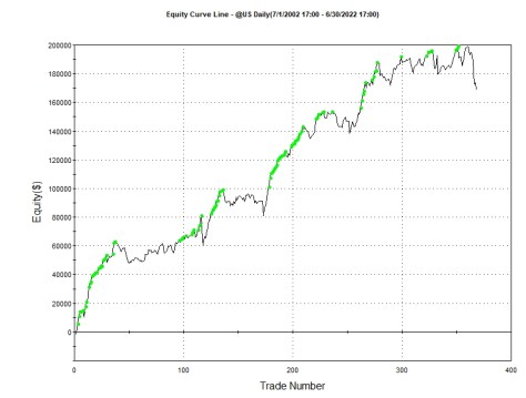
Not a bad equity curve. To be fair to Murray he did notice the connection between $UTY and the bonds was changing over the past couple of year. And this simple stop and reverse system doesn’t have a protective stop. But it wouldn’t look much different with one, because the system looks at momentum of the primary data and momentum of the secondary data and if they are in synch (either positively or negatively correlated – selected by the algo) an order is fired off. If you simply just add a protective stop, and the momentum of the data are in synch, the strategy will just re-enter on the next bar. However, the equity curve just made a new high recently. It has got on the wrong side of the Fed raising rates. One could argue that this invisible hand has toppled the apple cart and this inter-market relationship has been rendered meaningless.

Murray had evolved his inter-market analysis to include state transitions. He not only looked at the current momentum, but also at where the momentum had been. He assigned the transitions of the momentum for the primary and secondary markets a value from one to four and he felt this state transition helped overcome some of the coupling/decoupling of the inter-market relationship.

However, I wanted to test Murray’s simple strategy with a fixed $ stop and force the primary market to move from positive to negative or negative to positive territory while the secondary market is in the correct relationship. Here is an updated equity curve.

George’s Adaptation and using a $4500 stop loss

This equity curve was developed by using a $4500 stop loss. Because I changed the order triggers, I reoptimized the length of the momentum calculations for the primary and secondary markets. This curve is only better in the category of maximum draw down. Shouldn’t we give Murray a chance and reoptimize his momentum length calculations too! You bet.

These metrics were sorted by Max Intraday Draw down. The numbers did improve, but look at the Max Losing Trade value. Murray’s later technology, his State Systems, were a great improvement over this basic system. Here is my optimization using a slightly different entry technique and a $4500 protective stop.

This system, using Murray’s overall research, achieved a better Max Draw Down and a much better Max Losing Trade. Here is my code using the template that Murray provided in his articles in Futures Magazine and EasyLanguage Mastery.

// Code by Murray Ruggiero
// adapted by George Pruitt

Inputs: InterSet(2),LSB(0),Type(1),LenTr(4),LenInt(4),Relate(0);
Vars: MarkInd(0),InterInd(0);

If Type=0 Then 
Begin
	InterInd=Close of Data(InterSet)-CLose[LenInt] of Data(InterSet);
	MarkInd=CLose-CLose[LenTr];
end;

If Type=1 Then 
Begin
	InterInd=Close of Data(InterSet)-Average(CLose of Data(InterSet),LenInt);
	MarkInd=CLose-Average(CLose,LenTr);
end;

if Relate=1 then 
begin
	If InterInd > 0 and MarkInd CROSSES BELOW 0 and LSB>=0 then 
		Buy("GO--Long") Next Bar  at open;
	If InterInd < 0 and MarkInd CROSSES ABOVE 0 and LSB<=0 then
		Sell Short("GO--Shrt") Next Bar  at open;

end;
if Relate=0 then begin
	If InterInd<0 and MarkInd CROSSES BELOW 0  and LSB>=0 then 
		Buy Next Bar  at open;
	If InterInd>0 and MarkInd CROSSES ABOVE 0  and LSB<=0 then 
		Sell Short Next Bar  at open;
end;

Here the user can actually include more than two data streams on the chart. The InterSet input allows the user to choose or optimize the secondary market data stream. Momentum is defined by two types:

Type 0: Intermarket or secondary momentum simply calculated by close of data(2) – close[LenInt] of date(2) and primary momentum calculated by close – close[LenTr]
Type 1: Intermarket or secondary momentum calculated by close of data(2) – average( close of data2, LenInt) and primary momentum calculated by close – average(close, LenTr)

The user can also input what type of Relationship: 1 for positive correlation and 0 for negative correlation. This template can be used to dig deeper into other market relationships.

George’s Modification

I simply forced the primary market to CROSS below/above 0 to initiate a new trade as long the secondary market was pointing in the right direction.

	If InterInd > 0 and MarkInd CROSSES BELOW 0 and LSB>=0 then 
		Buy("GO--Long") Next Bar  at open;
	If InterInd < 0 and MarkInd CROSSES ABOVE 0 and LSB<=0 then
		Sell Short("GO--Shrt") Next Bar  at open;

Using the keyword CROSSES

This was a one STATE transition and also allowed a protective stop to be used without the strategy automatically re-entering the trade in the same direction.

Thank You Murray – we sure do miss you!

Murray loved to share his research and would want us to carry on with it. I will write one or two blogs a year in tribute to Murray and his invaluable research.

Super Trend Indicator in EasyLanguage

February 27, 2022 George Pruitt Leave a comment

SuperTrend Indicator – What Is It?

SuperTrend is a trading strategy and indicator all built into one entity. There are a couple of versions floating around out there. MultiCharts and Sierra Chart both have slightly different flavors of this combo approach.

Ratcheting Trailing Stop Paradigm

This indic/strat falls into this category of algorithm. The indicator never moves away from your current position like a parabolic stop or chandelier exit. I used the code that was disclosed on Futures.io or formerly known as BigMikesTrading blog. This version differs from the original SuperTrend which used average true range. I like Big Mike’s version so it will discussed here.

Big Mike’s Math

The math for this indicator utilizes volatility in the terms of the distance the market has travelled over the past N days. This is determined by calculating the highest high of the last N days/bars and then subtracting the lowest low of last N days/bars. Let’s call this the highLowRange. The next calculation is an exponential moving average of the highLowRange. This value will define the market volatility. Exponential moving averages of the last strength days/bars highs and lows are then calculated and divided by two – giving a midpoint. The volatility measure (multiplied my mult) is then added to this midpoint to calculate an upper band. A lower band is formed by subtracting the volatility measure X mult from the midpoint.

Upper or Lower Channel?

If the closing price penetrates the upper channel and the close is also above the highest high of strength days/bars back (offset by one of course) then the trend will flip to UP. When the trend is UP, then the Lower Channel is plotted. Once the trend flips to DN, the upper channel will be plotted. If the trend is UP the lower channel will either rise with the market or stay put. The same goes for a DN trend – hence the ratcheting. Here is a graphic of the indicator on CL.

If you plan on using an customized indicator in a strategy it is always best to build the calculations inside a function. The function then can be used in either an indicator or a strategy.

Function Name: SuperTrend_BM

Function Type: Series – we will need to access prior variable values

SuperTrend_BM Function Code:

//SuperTrend from Big Mike now futures.io

inputs: 
length(NumericSimple), mult(NumericSimple), strength(NumericSimple), STrend(NumericRef);

vars: 
highLowRange(0), 
xAvgRng(0),
xAvg(0), 
dn(0), 
up(0), 
trend(1), 
trendDN(False), 
trendUP(False), 
ST(0); 

highLowRange = Highest(high, length) - Lowest(low, length);

xAvgRng = XAverage(highLowRange, length);

xAvg = (XAverage(high, Strength) + XAverage(low, Strength))/2;

up = xAvg + mult * xAvgRng; 
dn = xAvg - mult * xAvgRng; 

if c > up[1] and c > Highest(High, strength)[1] then
	trend = 1
else 
	if c < dn[1] and c < Lowest(Low, Strength)[1] then
		trend = -1;

//did trend flip?		
trendDN = False;
trendUP = False;

if trend < 0 and trend[1] > 0 then 
	trendDN	= True; 	
if trend > 0 and trend[1] < 0 then 
	trendUP = True;
	
//ratcheting mechanism
if trend > 0 then dn = maxList(dn,dn[1]);
if trend < 0 then up = minList(up,up[1]);

// if trend dir. changes then assign
// up and down appropriately
if trendUP then
	up = xAvg + mult * xAvgRng; 	
if trendDN then
	dn = xAvg - mult * xAvgRng; 

if trend = 1 then 
	ST = dn 
else
	ST = up;
	
STrend = trend;

SuperTrend_BM = ST;

SuperTrend ala Big Mike

The Inputs to the Function

The original SuperTrend did include the Strength input. This input is a Donchian like signal. Not only does the price need to close above/below the upper/lower channel but also the close must be above/below the appropriate Donchian Channels to flip the trend, Also notice we are using a numericRef as the type for STrend. This is done because we need the function to return two values: trend direction and the upper or lower channel value. The appropriate channel value is assigned to the function name and STrend contains the Trend Direction.

A Function Driver in the Form of an Indicator

A function is a sub-program and must be called to be utilized. Here is the indicator code that will plot the values of the function using: length(9), mult(1), strength(9).

// SuperTrend indicator
// March 25 2010
// Big Mike https://www.bigmiketrading.com 
inputs: 
length(9), mult(1), strength(9);

vars: 
strend(0),
st(0);

st = SuperTrend_BM(length, mult,strength,strend);

if strend = 1 then Plot1(st,"SuperTrendUP");
if strend = -1 then Plot2(st,"SuperTrendDN");

Function Drive in the form of an Indicator

This should be a fun indicator to play with in the development of a trend following approach. My version of Big Mike’s code is a little different as I wanted the variable names to be a little more descriptive.

Update Feb 28 2022

I forgot to mention that you will need to make sure your plot lines don’t automatically connect.

Can You Do This with Just One Plot1?

An astute reader brought it to my attention that we could get away with a single plot and he was right. The reason I initially used two plot was to enable the user to chose his/her own plot colors by using the Format dialog.

//if strend = 1 then Plot1(st,"SuperTrendUP");
//if strend = -1 then Plot2(st,"SuperTrendDN");

if strend = 1 then SetPlotColor(1,red);
if strend = -1 then SetPlotColor(1,green);

Plot1(st,"SuperTrend_BM");

Method to just use one Plot1

Complete EasyLanguage Systems, EasyLanguage, EasyLanguage Object, EasyLanguage Snippets, EasyLanguage Tutorial, EasyLanguage Tutorial, Must Know, Must Know EasyLanguage, OOEL

Tracking Last EntryPrice While Pyramiding on Minute Bars

January 25, 2022 George Pruitt Leave a comment

EasyLanguage’s EntryPrice Doesn’t Cut the Mustard

In writing the Hi-Res edition of Easing Into EasyLanguage I should have included this sample program. I do point out the limitations of the EntryPrice keyword/function in the book. But recently I was tasked to create a pyramiding scheme template that used minute bars and would initiate a position with N Shares and then pyramid up to three times by adding on N Shares at the last entry price + one 10 -Day ATR measure as the market moves in favor of the original position. Here is an example of just such a trade.

Pyramid 3 Times After Initial Trade Entry. Where’s the EntryPrice?

EntryPrice only contains the original entry price. So every time you add on a position, the EntryPrice doesn’t reflect this add on price. I would like to be able to index into this keyword/function and extract any EntryPrice. If you enter at the market, then you can keep track of entry prices because a market order is usually issued from an if-then construct:

//Here I can keep track of entry prices because I know
//exactly when and where they occur.

if c > c[1] and value1 > value2 then
begin
	buy("MarketOrder") next bar at market;
	lastEntryPrice = open of next bar;
end;

Last Entry Price tracking is easy if using Market Orders

But what if you are using a stop or limit order. You don’t know ahead of time where one of these types of orders will hit up. It could be the next bar or it could be five bars later or who knows.

AvgEntryPrice Makes Up for the Weakness of EntryPrice

AvgEntryPrice is a keyword/function that returns the average of the entries when pyramiding. Assume you buy at 42.00 and pyramid the same number of shares at 46.50 – AvgEntryPrice will be equal to (42.00 + 46.50) / 2 = 44.25. With this information you can determine the two entry prices. You already know the original price. Take a look at this code.

// remember currentShares and avgEntryPrice ARE EasyLanguage Keywords/Functions
if mp[1] = mp and mp = -1 and currentShares > curShares then
begin
	totShorts = totShorts + 1;
	if currentShares > initShares then
	begin
		lastEntryPrice = totShorts * avgEntryPrice - entryPriceSums;
		entryPriceSums = entryPriceSums + lastEntryPrice;
		print(d," Short addon ",lastEntryPrice," ",totShorts," ",avgEntryPrice," ",entryPriceSums);
	end;
end;

Calculating the true LastEntryPrice

Remember currentShares is a keyword/function and it is immediately updated when more shares are added or taken off. CurShares is my own variable where I keep track of the prior currentShares , so if currentShares (real number of shares) is greater than the prior curShares (currentShares) then I know 100%, a position has been pyramided as long the the mp stays the same. If currentShares increases and mp stays constant, then you can figure out the last entry price where the pyramid takes place. First you tick totShorts up by 1. If currentShares > initShares, then you know you are pyramiding so

lastEntryPrice = totShorts * avgEntryPrice – entryPriceSums

Don’t believe me. Let’s test it. Remember original entry was 42.00 and the add on was at 46.50. TotShorts now equals 2.

Initial entryPrice = 42.00 so entryPriceSums is set to 42.00
After pyramiding avgEntryPrice is set to 44.25
lastEntryPrice = 2 * 44.25 – 42.00 = 46.50
entryPriceSums is then set to 42.00 + 46.50 or 88.50

So every time you add on a position, then you flow through this logic and you can keep track of the actual last entry price even if it is via a limit or stop order.

But wait there is more. This post is also a small glimpse into what I will be writing about in the Easing Into EasyLanguage: Advanced Topics. This system definitely falls into what I discussed in the Hi-Res Edition. Here is where we tip over into Advanced Topics. The next book is not about creating dialogs or trading apps using OOEL (object oriented EasyLanguage), but we do use some of those topics to do some rather complicated back testing things.

Now that we know how to calculate the lastEntryPrice wouldn’t it be really cool if we could keep track of all of the entryPrices during the pyramid stream. If I have pyramided four times, I would like to know entryPrice 1, entryPrice 2, entryPrice 3 and entryPrice 4.

Dr. VectorLove or How I Learned to Stop Worrying and Love Objects

I have discussed vectors before but I really wanted to discuss them more. Remember Vectors are just lists or arrays that don’t need all the maintenance. Yes you have to create them which can be a pain, but once you learn and forget it twenty times it starts to sink in. Or just keep referring back to this web page.


Using elsystem.collections;

vars: Vector entryPriceVector(Null);

once Begin
	entryPriceVector = new Vector;
end;

The Bare Minimum to Instantiate a Vector

Type – “Using elsystem.collections; “
Declare entryPriceVector as a Vector and set it equal to Null
Use Once and instantiate entryPriceVector by using the keyword new < object type>;

A Vector is part of elsystem’s collection objects. Take a look at this updated code,

if mp[1] = mp and mp = -1 and currentShares > curShares then
begin
	totShorts = totShorts + 1;
	if currentShares > initShares then
	begin
		lastEntryPrice = totShorts * avgEntryPrice - entryPriceSums;
		entryPriceVector.push_back(lastEntryPrice);
		entryPriceSums = entryPriceSums + lastEntryPrice;
		print(d," Short addon ",lastEntryPrice," ",entryPrice," ",entryPrice(1)," ",totShorts," ",avgEntryPrice," ",entryPriceSums," ",entryPriceVector.back() astype double," ",entryPriceVector.count asType int);
		if not(entryPriceVector.empty()) then
		begin
			for m = 0 to entryPriceVector.count-1
			begin
				print(entryPriceVector.at(m) astype double);
			end;
		end;
	end;
end;

LastEntryPrice and Pushing It onto the Vector and Then Printing Out the Vector

After the lastEntryPrice is calculated it is pushed onto the entryPriceVector using the function (method same thing but it is attached to the Vector class).push_back(lastEntryPrice);

entryPriceVector.push_back(lastEntryPrice);

So every time a new lastEntryPrice is calculated it is pushed onto the Vector at the back end. Now if the entryPriceVector is not empty then we can print its contents by looping and indexing into the Vector.

if not(entryPriceVector.empty()) then
begin
     for m = 0 to entryPriceVector.count-1
     begin
          print(entryPriceVector.at(m) astype double);
     end;
end;

Looping through a Vector and Printing Out its Contents

Remember if you NOT a boolean value then it turns it to off/on or just the opposite of the boolean value. If entryPriceVector is not empty then proceed. entryPriceVector.count holds the number of values stuffed into the vector. You can index into the Vector by using .at(m), If you want to print out the value of the Vector .at(m), then you will need to typecast the Vector object as what ever it is holding. We know we are pushing numbers with decimals (double type) onto the Vector so we know we can evaluate them as a double type. Just remember you have to do this when printing out the values of the Vector.

Okay you can see where we moved into an Advanced Topics area with this code. But it really becomes useful when trying to overcome some limitations of EasyLanguage. Remember keep an eye open for Advanced Topics sometime in the Spring.