Category Archives: EasyLanguage Snippets

Can Futures Traders Trust Continuous Contracts? [Part – 1]

 Well You Have To, Don’t You?

When I worked at Futures Truth, we tested everything with our Excalibur software.  This software used individual contract data and loaded the entire history (well, the part we maintained) of each contract into memory and executed rollovers at a certain time of the month.  Excalibur had its limitations as certain futures contracts had very short histories and rollover dates had to be predetermined – in other words, they were undynamic.  Over the years, we fixed the short history problem by creating a dynamic continuous contract going back in time for the number of days required for a calculation.  We also fixed the database with more appropriate rollover frequency and dates.  So in the end, the software simulated what I had expected from trading real futures contracts.  This software was originally written in Fortran and for the Macintosh.  It also had limitations on portfolio analysis as it worked its way across the portfolio, one complete market at a time.   Even with all these limitations, I truly thought that the returns more closely mirrored what a trader might see in real time.  Today, there aren’t many, if any, simulation platforms that test on individual contracts.  The main reasons for this are the complexity of the software, and the database management.  However, if you are willing to do the work, you can get close to testing on individual contract data with EasyLanguage.

Step 1 – Get the rollover dates

This is critical as the dates will be used to roll out of one contract and into another.  In this post, I will test a simple strategy on the crude futures.  I picked crude because it rolls every month.   Some data vendors use a specific date to roll contracts, such as Pinnacle data.  In real time trading, I did this as well.  We had a calendar for each month, and we would mark the rollover dates for all markets traded at the beginning of each month.  Crude was rolled on the 11th or 12th of the prior month to expiration.  So, if we were trading the September 2022 contract, we would roll on August 11th.  A single order (rollover spread) was placed to sell (if long) the September contract and buy the October contract at the market simultaneously.  Sometimes we would leg into the rollover by executing two separate orders – in hopes of getting better execution.  I have never been able to find a historic database of when TradeStation performs its rollovers.  When you use the default @CL symbol, you allow TradeStation to use a formula to determine the best time to perform a rollover.  This was probably based on volume and open interest.  TradeStation does allow you to pick several different rollover triggers when using their continuous data.

You can choose type of trigger – (3) Dynamic or (4) Time based.

I am getting ahead of myself, because we can simply use the default @CL data to derive the rollover dates (almost.)  Crude oil is one of those weird markets where LTD (last trade days) occurs before FND (first notice day.)  Most markets will give you a notice before they back up a huge truck and dump a 1000 barrels of oil at your front door.   With crude you have to be Johnny on the spot!  Rollover is just a headache when trading futures, but it can be very expensive headache if you don’t get out in time.  Some markets are cash settled so rollover isn’t that important, but others result in delivery of the commodity.  Most clearing firms will help you unwind an expired contract for a small fee (well relatively small.)  In the good old days your full service broker would give you heads up.  They would call you and say, “George you have to get out of that Sept. crude pronto!”  Some firms would automatically liquidate the offending contract on your behalf – which sounds nice but it could cost you.  Over my 30 year history of trading futures I was caught a few times in the delivery process.   You can determine these FND and LTD from the CME website.  Here is the expiration description for crude futures.

Trading terminates 3 business day before the 25th calendar day of the month prior to the contract month. If the 25th calendar day is not a business day, trading terminates 4 business days before the 25th calendar day of the month prior to the contract month.

You can look this up on your favorite broker’s website or the handy calendars they send out at Christmas.  Based on this description, the Sept. 2022 Crude contract would expire on August 20th and here’s why

  • August 25 is Tuesday
  • August 24 is Monday- DAY1
  • August 21 is Friday – DAY2
  • August 20 is Thursday – DAY3

This is the beauty of a well oiled machine or exchange.  The FND will occur exactly as described.  All you need to do is get all the calendars for the past ten years and find the 25th of the month and count back three business days.  Or if the 25 falls on a weekend count back four business days.  Boy that would be chore, would it not?  Luckily, we can have the data and an  EasyLanguage script do this for us.  Take a look at this code and see if it makes any sense to you.

Case "@CL":
If dayOfMonth(date) = 25 and firstMonthPrint = false then
begin
print(date[3]+19000000:8:0);
firstMonthPrint = true;
end;
If(dayOfMonth(date[1]) < 25 and dayOfMonth(date) > 25 ) and firstMonthPrint = false then
begin
print(date[4]+19000000:8:0);
firstMonthPrint = true;
end;
Code to printout all the FND of crude oil.

I have created a tool to print out the FND or LTD of any commodity futures by examining the date.  In this example, I am using a Switch-Case to determine what logic is applied to the chart symbol.  If the chart symbol is @CL, I look to see if the 25th of the month exists and if it does, I print the date 3 days prior out.  If today’s day of month is greater than 25 and the prior day’s day of month is less than 25, I know the 25th occurred on a weekend and I must print out the date four bars prior.  These dates are FN dates and cannot be used as is to simulate a rollover. You had best be out before the FND to prevent the delivery process.   Pinnacle Date rolls the crude on the 11th day of the prior month for its crude continuous contracts.  I aimed for this day of the month with my logic.  If the FND normally fell on the 22nd of the month, then I should back up either 9 or 10 business days to get near the 11th of the month.   Also I wanted to use the output directly in an EasyLanguage strategy so I modified my output to be exact EasyLanguage.

Case "@CL":
If dayOfMonth(date) = 25 and firstMonthPrint = false then
begin
value1 = value1 + 1;
print("rollArr[",value1:1:0,"]=",date[9]+19000000:8:0,";");
firstMonthPrint = true;
end;
If(dayOfMonth(date[1]) < 25 and dayOfMonth(date) > 25 ) and firstMonthPrint = false then
begin
value1 = value1 + 1;
print("rollArr[",value1:1:0,"]=",date[10]+19000000:8:0,";");
// print(date[4]+19000000:8:0);
firstMonthPrint = true;
end;


// example of output

rollArr[103]=20210312;
rollArr[104]=20210412;
rollArr[105]=20210512;
rollArr[106]=20210614;
rollArr[107]=20210712;
rollArr[108]=20210812;
rollArr[109]=20210913;
rollArr[110]=20211012;
rollArr[111]=20211111;
rollArr[112]=20211210;
rollArr[113]=20220111;
rollArr[114]=20220211;
rollArr[115]=20220314;
rollArr[116]=20220411;
rollArr[117]=20220512;
rollArr[118]=20220610;
rollArr[119]=20220712;
rollArr[120]=20220812;
Code to print our 9 or 10 bars prior to FND in actual EasyLanguage

Now. that I had the theoretical rollover dates for my analysis I had to make sure the data that I was going to use matched up exactly.  As you saw before, you can pick the rollover date for your chart data.   And you can also determine the discount to add or subtract to all prior data points based on the difference between the closing prices at the rollover point.  I played around with the number of days prior to FND and selected non adjusted for the smoothing of prior data.

Actual data I simulated rollovers with.

How did I determine 8 days Prior to First Notice Date?  I plotted different data using a different number of days prior and determined 8 provided a sweet spot between the old and new contract data’s open interest.  Can you see the rollover points in the following chart?  Ignore the trades – these were a beta test.

The Open Interest Valley is the rollover date.

The dates where the open interest creates a valley aligned very closely with the dates I printed out using my FND date finder function.  To be safe, I compared the dates and fixed my array data to match the chart exactly.  Here are two rollover trades – now these are correct.

Using an adjusted continuous contract you would not see these trades.

This post turned out to be a little longer than I thought, so I will post the results of using an adjusted continuous contract with no rollovers, and the results using non-adjusted concatenated contracts with rollovers.  The strategy will be a simple 40/20 bar Donchian entry/exit.  You maybe surprised by the results – stay tuned.

A Tribute to Murray and His Inter-Market Research

Murray Ruggiero’s Inter-Market Research

Well it’s been a year, this month, that Murray passed away.  I was fortunate to work with him on many of his projects and learned quite a bit about inter-market convergence and divergence.  Honestly, I wasn’t that into it, but you couldn’t argue with his results.  A strategy that he developed in the 1990s that compared the Bond market with silver really did stand the test of time.  He monitored this relationship over the years and watched in wane.  Murray replaced silver with $UTY.

The PHLX Utility Sector Index (UTY) is a market capitalization-weighted index composed of geographically diverse public utility stocks.

He wrote an article for EasyLanguage Mastery by Jeff Swanson where he discussed this relationship and the development of inter-market strategies and through statistical analysis proved that these relationships added real value.

I am currently writing Advanced Topics, the final book in my Easing Into EasyLanguage trilogy, and have been working with Murray’s research.  I am fortunate to have a complete collection of his Futures Magazine articles from the mid 1990s to the mid 2000s.  There is a quite a bit of inter-market stuff in his articles.  I wanted, as a tribute and to proffer up some neat code, to show the performance and code of his Bond and $UTY inter-market algorithm.

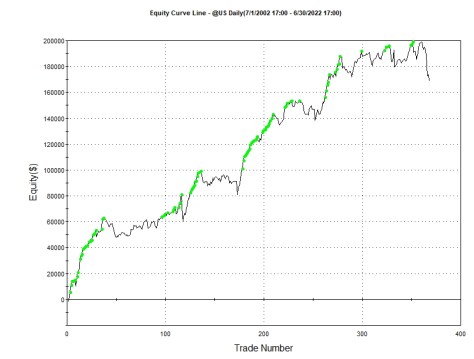
Here is a version that he published a few years ago updated through June 30, 2022 – no commission/slippage.

Murray’s Bond and $UTY inter-market Strategy

Not a bad equity curve.  To be fair to Murray he did notice the connection between $UTY and the bonds was changing over the past couple of year.  And this simple stop and reverse system doesn’t  have a protective stop.   But it wouldn’t look much different with one, because the system looks at momentum of the primary  data and momentum of the secondary data and if they are in synch (either positively or negatively correlated – selected by the algo) an order is fired off.  If you simply just add a protective stop, and the momentum of the data are in synch, the strategy will just re-enter on the next bar.  However, the equity curve just made a new high  recently.  It has got on the wrong side of the Fed raising rates.  One could argue that this invisible hand has toppled the apple cart and this inter-market relationship has been rendered meaningless.

Murray had evolved his inter-market analysis to include state transitions.  He not only looked at the current momentum, but also at where the momentum had been.  He assigned the transitions of the momentum for the primary and secondary markets a value from one to four and he felt this state transition helped overcome some of the coupling/decoupling of the inter-market relationship.

However,  I wanted to test Murray’s simple strategy with a fixed $ stop and force the primary market to move from positive to negative or negative to positive territory while the secondary market is in the correct relationship.  Here is an updated equity curve.

George’s Adaptation and using a $4500 stop loss

This equity curve was developed  by using a $4500 stop loss.  Because I changed the order triggers, I reoptimized the length of the momentum calculations for the primary and secondary markets.  This curve is only better in the category of maximum draw down.  Shouldn’t we give Murray a chance and reoptimize his momentum length calculations too!  You bet.

Murray Length Optimizations

These metrics were sorted by Max Intraday Draw down.  The numbers did improve, but look at the Max Losing Trade value.  Murray’s later technology,  his State Systems, were a great improvement over this basic system.  Here is my optimization using a slightly different entry technique and a $4500 protective stop.

Standing on the Shoulders of a Giant

This system, using Murray’s overall research, achieved a better Max Draw Down and a much better Max Losing Trade.   Here is my code using the template that Murray provided in his articles in Futures Magazine and EasyLanguage Mastery.


// Code by Murray Ruggiero
// adapted by George Pruitt

Inputs: InterSet(2),LSB(0),Type(1),LenTr(4),LenInt(4),Relate(0);
Vars: MarkInd(0),InterInd(0);

If Type=0 Then
Begin
InterInd=Close of Data(InterSet)-CLose[LenInt] of Data(InterSet);
MarkInd=CLose-CLose[LenTr];
end;

If Type=1 Then
Begin
InterInd=Close of Data(InterSet)-Average(CLose of Data(InterSet),LenInt);
MarkInd=CLose-Average(CLose,LenTr);
end;

if Relate=1 then
begin
If InterInd > 0 and MarkInd CROSSES BELOW 0 and LSB>=0 then
Buy("GO--Long") Next Bar at open;
If InterInd < 0 and MarkInd CROSSES ABOVE 0 and LSB<=0 then
Sell Short("GO--Shrt") Next Bar at open;

end;
if Relate=0 then begin
If InterInd<0 and MarkInd CROSSES BELOW 0 and LSB>=0 then
Buy Next Bar at open;
If InterInd>0 and MarkInd CROSSES ABOVE 0 and LSB<=0 then
Sell Short Next Bar at open;
end;

Here the user can actually include more than two data streams on the chart.  The InterSet input allows the user to choose or optimize the secondary market data stream.  Momentum is defined by two types:

  • Type 0:  Intermarket or secondary momentum simply calculated by close of data(2) – close[LenInt] of date(2) and primary momentum calculated by close – close[LenTr]
  • Type 1:   Intermarket or secondary momentum  calculated by close of data(2) – average( close of data2, LenInt)  and primary momentum calculated by close – average(close, LenTr)

The user can also input what type of Relationship: 1 for positive correlation and 0 for negative correlation.  This template can be used to dig deeper into other market relationships.

George’s Modification

I simply forced the primary market to CROSS below/above 0 to initiate a new trade as long the secondary market was pointing in the right direction.

	If InterInd > 0 and MarkInd CROSSES BELOW 0 and LSB>=0 then 
Buy("GO--Long") Next Bar at open;
If InterInd < 0 and MarkInd CROSSES ABOVE 0 and LSB<=0 then
Sell Short("GO--Shrt") Next Bar at open;
Using the keyword CROSSES

This was a one STATE transition and also allowed a protective stop to be used without the strategy automatically re-entering the trade in the same direction.

Thank You Murray – we sure do miss you!

Murray loved to share his research and would want us to carry on with it.  I will write one or two blogs a year in tribute to Murray and his invaluable research.

Using EXCEL VBA to Combine Equity Curves from TradeStation

A Poor Man’s Equity Curve Merger

Sometimes you just want to create a combined equity curve of several markets and for one reason or another you don’t want to use Maestro.  This post will show you an indicator that you can insert into your TradeStation chart/strategies that will output monthly cumulative equity readings.  After that I refresh my VBA skills a little bit by creating a VBA Macro/Script that will take the output and parse it into a table where the different months are the rows and the different market EOM equities, for those months, will be the columns.  Then all the rows will be summed and then finally a chart will be produced.  I will zip the Exel .xlsm and include it at the end of this post.

Part 1:  Output Monthly Data to Print Log

You can determine the end of the month by comparing the current month of the date and the month of the prior date.  If they are different, then you know you are sitting on the first trading day of the new month.  You can then reach back and access the total equity as of yesterday.  If you want you can also track the change in month equity.  Here is the indicator code in EasyLanguage.

// Non plotting indicator that needs to be applied to 
// a chart that also has a strategy applied
// one that produces a number of trades

vars: monthlyEqu(0),priorMonthEqu(0);
vars: totalEquity(0);


if month(date) <> month(date[1]) then
begin
monthlyEqu = totalEquity[1] - priorMonthEqu;
priorMonthEqu = totalEquity[1];
print(getSymbolName,",",month(date[1]):2:0,"-",year(date[1])+1900:4:0,",",monthlyEqu,",",totalEquity);
end;
totalEquity = i_ClosedEquity;
Indicator that exports the EOM equity values

The interesting part of this code is the print statement.  You can use the month and year  functions to extract the respective values from the date bar array.  I use a formatted print to export the month and year without decimals.  Remember 2021 in TradeStation is represented by 121 and all you have to do is add 1900 to get a more comfortable value.  The month output is formatted with :2:0 and the year with :4:0.  The first value in the format notation informs  the computer to allow at least 2 or 4 values for the month  and the year respectively.  The second value following the second colon informs the computer that you do not want any decimals values (:0).  Next insert the indicator into all the charts in your workspace.  Here’s a snippet of the output on one market.  I tested this on six markets and this data was the output generated.  Some of the markets were interspersed and that is okay.  You may have a few months of @EC and then a few months of @JY and then @EC again.

@EC, 7-2008,-5106.24,-5106.24
@EC, 8-2008, 0.00,-5106.24
@EC, 9-2008, 0.00,-5106.24
@EC,10-2008, 0.00,-5106.24
@EC,11-2008, 0.00,-5106.24
@EC,12-2008,25156.26,20050.02
@EC, 1-2009, 0.00,20050.02
@EC, 2-2009, 0.00,20050.02
@EC, 3-2009, 0.00,20050.02
@EC, 4-2009, 0.00,20050.02
@EC, 5-2009, 0.00,20050.02
@EC, 6-2009, 0.00,20050.02
@EC, 7-2009, 0.00,20050.02
@EC, 8-2009, 0.00,20050.02
@EC, 9-2009, 0.00,20050.02
@EC,10-2009, 0.00,20050.02
@EC,11-2009, 0.00,20050.02
@EC,12-2009,7737.51,27787.53
@EC, 1-2010, 0.00,27787.53
@EC, 2-2010, 0.00,27787.53
@EC, 3-2010, 0.00,27787.53
@EC, 4-2010, 0.00,27787.53
@EC, 5-2010, 0.00,27787.53
@EC, 6-2010, 0.00,27787.53
@EC, 7-2010, 0.00,27787.53
@EC, 8-2010, 0.00,27787.53
@EC, 9-2010,6018.76,33806.29
Indicator output

Part 2: Getting the Data into Excel

If you use this post’s EXCEL workbook with the macro you may need to tell EXCEL to forget any formatting that might already be inside the workbook.  Open my workbook and beware that it will inform/warn you that a macro is located inside and that it could be dangerous.  If you want to go ahead and enable the macro go ahead.  On Sheet1 click in A1 and place the letter “G”.  Then goto the Data Menu and then the Data Tools section of the ribbon and click Text to Columns.  A dialog will open and ask you they type of file that best describes your data.  Click the Delimited radio button and then next.  You should see a dialog like this one.

Clear Any Left Over Formatting

Now copy all of the data from the Print-Log and paste it into Column A.  If all goes right everything will be dumped in the appropriate rows and in a single column.

The fields will be dumped into a single column

First select column A and  go back to the Data Menu and the Data Tools on the Ribbon.  Select Delimited and hit next,  Choose comma because we used commas to separate our values.  Click Next again.  Eventually you will get to this dialog.

Make sure you use Date [MDY] for the second column of data.
If you chose Date format for column 2 with MDY, then it will be imported into the appropriate column in a date format.  This makes charting easier.  If all goes well then you will have four columns of data –  a column for Symbol, Date, Delta-EOM and EOM.  Select column B and right click and select Format Cells.

Clean Up column B by formatting cells and customizing the date format

Once you format the B column in the form of  MM-YYYY you will have a date like 9-2007, 10-2007, 11-2007…

Running the VBA Macro/Script

On the Ribbon in EXCEL goto the Developer Tab.  If you don’t see it then you will need to install it.  Just GOOGLE it and follow their instructions.  Once on the Develop Tab goto the Code category and click the Visual Basic Icon.  Your VBA IDE will open and should like very similar to this.

VBA IDE [integrated development environment]
If all goes according to plan after you hit the green Arrow for the Run command your spreadsheet should like similar to this.

EOM table with Months as Rows and Individual Market EOMs as columns

The Date column will be needed to be reformatted again as Date with Custom MM-YYYY format.  Now copy the table by highlighting the columns and rows including the headings and then goto to Insert Menu and select the Charts category.  

This is what you should get.

Merged Equity on Closed Trade Basis

This is the output of the SuperTurtle Trading system tested on the currency sector from 2007 to the present.

VBA Code

I have become very spoiled using Python as it does many things for you by simply calling a function.  This code took my longer to develop than I thought it would, because I had to back to the really old school of programming (really wanted to see if I could do this from scratch) to get this done.  You could of course eliminate some of my code by calling spread sheet functions from within EXCEL.  I went ahead and did it the brute force way just to see if I could do it.

Sub combineEquityFromTS()

'read data from columns
'symbol, date, monthlyEquity, cumulativeEquity - format
'create arrays to hold each column of data
'use nested loops to do all the work
'brute force coding, no objects - just like we did in the 80s

Dim symbol(1250) As String
Dim symbolHeadings(20) As String
Dim myDate(1250) As Long
Dim monthlyEquity(1250) As Double
Dim cumulativeEquity(1250) As Double

'read the data from the cells
dataCnt = 1
Do While Cells(dataCnt, 1) <> ""
symbol(dataCnt) = Cells(dataCnt, 1)
myDate(dataCnt) = Cells(dataCnt, 2)
monthlyEquity(dataCnt) = Cells(dataCnt, 3)
cumulativeEquity(dataCnt) = Cells(dataCnt, 4)
dataCnt = dataCnt + 1
Loop
dataCnt = dataCnt - 1

'get distinct symbolNames and use as headers
symbolHeadings(1) = symbol(1)
numSymbolheadings = 1
For i = 2 To dataCnt - 1
If symbol(i) <> symbol(i + 1) Then
newSymbol = True
For j = 1 To numSymbolheadings
If symbol(i + 1) = symbolHeadings(j) Then
newSymbol = False
End If
Next j
If newSymbol = True Then
numSymbolheadings = numSymbolheadings + 1
symbolHeadings(numSymbolheadings) = symbol(i + 1)
End If
End If
Next i

'Remove duplicate months in date array
'have just one column of month end dates

Cells(2, 7) = myDate(1)
dispRow = 2
numMonths = 1
i = 1
Do While i <= dataCnt
foundDate = False
For j = 1 To numMonths
If myDate(i) = Cells(j + 1, 7) Then
foundDate = True
End If
Next j
If foundDate = False Then
numMonths = numMonths + 1
Cells(numMonths + 1, 7) = myDate(i)
End If
i = i + 1
Loop
'put symbols across top of table
'put "date" and "cumulative" column headings in proper
'locations too

Cells(1, 7) = "Date"
For i = 1 To numSymbolheadings
Cells(1, 7 + i) = symbolHeadings(i)
Next i

numSymbols = numSymbolheadings
Cells(1, 7 + numSymbols + 1) = "Cumulative"
'now distribute the monthly returns in their proper
'slots in the table
dispRow = 2
dispCol = 7
For i = 1 To numSymbols
For j = 2 To numMonths + 1
For k = 1 To dataCnt
foundDate = False
If symbol(k) = symbolHeadings(i) And myDate(k) = Cells(j, 7) Then
Cells(dispRow, dispCol + i) = cumulativeEquity(k)
dispRow = dispRow + 1
Exit For
End If
'for later use
'If j > 1 Then
' If symbol(k) = symbolHeadings(i) And myDate(k) < Cells(j, 7) And myDate(k) > Cells(j - 1, 7) Then
' dispRow = dispRow + 1
' End If
'End If
Next k
Next j
dispRow = 2
Next i
'now accumulate across table and then down
For i = 1 To numMonths
cumulative = 0
For j = 1 To numSymbols
cumulative = cumulative + Cells(i + 1, j + 7)
Next j
Cells(i + 1, 7 + numSymbols + 1) = cumulative
Next i
End Sub

This a throwback to the 80s BASIC on many of the family computers of that era.  If you are new to VBA you can access cell values by using the keyword Cells and the row and column that points to the data.   The first thing you do is create a Module named combineEquityFromTS and in doing so it will create a Sub combineEquityFromTS() header and a End Sub footer.  All of your code will be squeezed between these two statements.  This code is ad hoc because I just sat down and started coding without much forethought.  

Use DIM to Dimension an Arrays

I like to read the date from the cells into arrays so I can manipulate the data internally.  Here I create five arrays and then loop through column one until there is no longer any data.  The appropriate arrays are filled with their respective data from each row.

Dimension and Load Arrays

Once the data is in arrays we can start do parse it.  The first thing I want is to get the symbolHeadings or markets.  I know the first row has a symbol name so I go ahead and put that into the symbolHeadings array.  I kept track of the number of rows in the data with the variable dataCnt.  Here I use  nested loops to work my way down the data and keep track of new symbols as I encounter them.  If the symbol changes values, I then check my list of stored symbolHeadings and if the new symbol is not in the list I add it.

Parse different symbols from all data

Since all the currencies will have the same month values I wanted to compress all the months into a single discrete month list.  This isn’t really all that necessary since we could have just prefilled the worksheet with monthly date values going back to 2007.  This algorithm is similar to the one that is used to extract the different symbols.  Except this time, just for giggles, I used a Do While Loop.

Squash Monthly List Down

As well as getting values from cells you can also put values into them.  Here I run through the list of markets and put them into Cells(1, 7+i).  When working with cells you need to make sure you get the offset correct.  Here I wanted to put the market names in Row A and Columns: H, I, J, K, L, M.

  • Column H = 8
  • Column I = 9
  • Column J = 10
  • Column K =11
  • Column L = 12
  • Column M = 13
Put Markets as Column Headers

Cells are two dimensional arrays.  However if you are going to use what is on the worksheet make sure you are referencing the correct data.  Here I introduce dispRow and dispCol as the anchor points where the data I need to reference starts out.

Three nested loops – Whopee.

Here I first parse through each symbol and extract the EOM value that matches the symbol name and month-year value.  So if I am working on @EC and I need the EOM for 07-2010, I fist loop through the month date values and compare the symbol AND myDate (looped through with another for-loop) with the month date values.  If they are the same then I dump the value in the array on to the spreadsheet.  And yes I should have used this:

For j = dispRow to numMonths-1

Instead of –

For j = 2 to numMonths-1

Keeping arrays in alignment with Cells can be difficult.  I have a hybrid approach here.  I will clean this up later and stick just with arrays and only use Cells to extract and place data.  The last thing you need to do is sum each row up and store that value in the Cumulative column.

Across and then Down to sum accumulated monthly returns

Conclusion

This was another post where we relied on another application to help us achieve our objective.   If you are new to EXCEL VBA (working with algorithms that generate trades) you can find out more in my Ultimate Algorithmic Trading System Toolbox book.  Even if you don’t get the book this post should get you started on the right track.

Excel Workbooks – One Empty with Macro and one Filled With this Post Data.


Tracking Last EntryPrice While Pyramiding on Minute Bars

EasyLanguage’s EntryPrice Doesn’t Cut the Mustard

In writing the Hi-Res edition of Easing Into EasyLanguage I should have included this sample program.  I do point out the limitations of the EntryPrice keyword/function in the book.  But recently I was tasked to create a pyramiding scheme template that used minute bars and would initiate a position with N Shares and then pyramid up to three times by adding on N Shares at the last entry price + one 10 -Day ATR measure as the market moves in favor of the original position.  Here is an example of just such a trade.

Pyramid 3 Times After Initial Trade Entry. Where’s the EntryPrice?

EntryPrice only contains the original entry price.  So every time you add on a position, the EntryPrice doesn’t reflect this add on price.  I would like to be able to index into this keyword/function and extract any EntryPrice.  If you enter at the market, then you can keep track of entry prices because a market order is usually issued from an if-then construct:

//Here I can keep track of entry prices because I know
//exactly when and where they occur.

if c > c[1] and value1 > value2 then
begin
buy("MarketOrder") next bar at market;
lastEntryPrice = open of next bar;
end;
Last Entry Price tracking is easy if using Market Orders

But what if you are using a stop or limit order.  You don’t know ahead of time where one of these types of orders will hit up.  It could be the next bar or it could be five bars later or who knows.

AvgEntryPrice Makes Up for the Weakness of EntryPrice

AvgEntryPrice is a keyword/function that  returns the average of the entries when pyramiding.  Assume you buy at 42.00 and pyramid the same number of shares at 46.50 – AvgEntryPrice will be equal to (42.00 + 46.50) / 2 = 44.25.  With this information you can determine the two entry prices.  You already know the original price.  Take a look at this code.

// remember currentShares and avgEntryPrice ARE EasyLanguage Keywords/Functions
if mp[1] = mp and mp = -1 and currentShares > curShares then
begin
totShorts = totShorts + 1;
if currentShares > initShares then
begin
lastEntryPrice = totShorts * avgEntryPrice - entryPriceSums;
entryPriceSums = entryPriceSums + lastEntryPrice;
print(d," Short addon ",lastEntryPrice," ",totShorts," ",avgEntryPrice," ",entryPriceSums);
end;
end;
Calculating the true LastEntryPrice

Remember currentShares is a keyword/function and it is immediately updated when more shares are added or taken off.  CurShares is my own variable where I keep track of the prior  currentShares , so if currentShares (real number of shares) is greater than the prior curShares (currentShares) then I know 100%, a position has been pyramided as long the the mp stays the same.  If currentShares increases and mp stays constant, then you can figure out the last entry price where the pyramid takes place.  First you tick totShorts up by 1.  If currentShares > initShares, then you know you are pyramiding so

lastEntryPrice = totShorts * avgEntryPrice – entryPriceSums

Don’t believe me.  Let’s test it.  Remember original entry was 42.00 and the add on was at 46.50.  TotShorts now equals 2.

  1. Initial entryPrice = 42.00 so entryPriceSums is set to 42.00
  2. After pyramiding avgEntryPrice is set to 44.25
  3. lastEntryPrice = 2 * 44.25 – 42.00 = 46.50
  4. entryPriceSums is then set to 42.00 + 46.50 or 88.50

So every time you add on a position, then you flow through this logic and you can keep track of the actual last entry price even if it is via a limit or stop order.

But wait there is more.  This post is also a small glimpse into what I will be writing about in the Easing Into EasyLanguage:  Advanced Topics.  This system definitely falls into what I discussed in the Hi-Res Edition.  Here is where we tip over into Advanced Topics.  The next book is not about creating dialogs or trading apps using OOEL (object oriented EasyLanguage), but we do use some of those topics to do some rather complicated back testing things.

Now that we know how to calculate the lastEntryPrice wouldn’t it be really cool if we could keep track of all of the entryPrices during the pyramid stream.   If I have pyramided four times, I would like to know entryPrice 1, entryPrice 2, entryPrice 3 and entryPrice 4.

EntryPrice Vector

Dr. VectorLove or How I Learned to Stop Worrying and Love Objects

I have discussed vectors before but I really wanted to discuss them more.  Remember Vectors are just lists or arrays that don’t need all the maintenance.  Yes you have to create them which can be a pain, but once you learn and forget it twenty times it starts to sink in.  Or just keep referring back to this web page.


Using elsystem.collections;

vars: Vector entryPriceVector(Null);

once Begin
entryPriceVector = new Vector;
end;
The Bare Minimum to Instantiate a Vector
  1. Type – “Using elsystem.collections; “
  2. Declare entryPriceVector as a Vector and set it equal to Null
  3. Use Once and instantiate entryPriceVector by using the keyword new < object type>;

A Vector is part of elsystem’s collection objects.  Take a look at this updated code,

if mp[1] = mp and mp = -1 and currentShares > curShares then
begin
totShorts = totShorts + 1;
if currentShares > initShares then
begin
lastEntryPrice = totShorts * avgEntryPrice - entryPriceSums;
entryPriceVector.push_back(lastEntryPrice);
entryPriceSums = entryPriceSums + lastEntryPrice;
print(d," Short addon ",lastEntryPrice," ",entryPrice," ",entryPrice(1)," ",totShorts," ",avgEntryPrice," ",entryPriceSums," ",entryPriceVector.back() astype double," ",entryPriceVector.count asType int);
if not(entryPriceVector.empty()) then
begin
for m = 0 to entryPriceVector.count-1
begin
print(entryPriceVector.at(m) astype double);
end;
end;
end;
end;
LastEntryPrice and Pushing It onto the Vector and Then Printing Out the Vector

After the lastEntryPrice is calculated it is pushed onto the entryPriceVector using the function (method same thing but it is attached to the Vector class).push_back(lastEntryPrice);

entryPriceVector.push_back(lastEntryPrice);

So every time a new lastEntryPrice is calculated it is pushed onto the Vector at the back end.  Now if the entryPriceVector is not empty then we can print its contents by looping and indexing into the Vector.

if not(entryPriceVector.empty()) then
begin
     for m = 0 to entryPriceVector.count-1
     begin
          print(entryPriceVector.at(m) astype double);
     end;
end;
Looping through a Vector and Printing Out its Contents

Remember if you NOT a boolean value then it turns it to off/on or just the opposite of the boolean valueIf entryPriceVector is not empty then proceed.  entryPriceVector.count holds the number of values stuffed into the vectorYou can index into the Vector by using .at(m),  If you want to print out the value of the Vector .at(m), then you will need to typecast the Vector object as what ever it is holding.  We know we are pushing numbers with decimals (double type) onto the Vector so we know we can evaluate them as a double type.  Just remember you have to do this when printing out the values of the Vector.

Okay you can see where we moved into an Advanced Topics area with this code.  But it really becomes useful when trying to overcome some limitations of EasyLanguage.  Remember keep an eye open for Advanced Topics sometime in the Spring.

Converting Method() To Function – MultiCharts

MultiCharts Doesn’t Support Methods

Methods are wonderful tools that are just like functions, but you can put them right into your Analysis Technique and they can share the variables that are defined outside the Method.  Here is an example that I have posted previously.  Note:  This was in response to a question I got on Jeff Swanson’s EasyLanguage Mastery Facebook Group.

{'('  Expected line 10, column 12  }
//the t in tradeProfit. // var: double tradeProfit;

vars: mp(0);
array: weekArray[5](0);


method void dayOfWeekAnalysis() {method definition}
var: double tradeProfit;
begin
If mp = 1 and mp[1] = -1 then tradeProfit = (entryPrice(1) - entryPrice(0))*bigPointValue;
If mp = -1 and mp[1] = 1 then tradeProfit = (entryPrice(0) - entryPrice(1))*bigPointValue;
weekArray[dayOfWeek(entryDate(1))] = weekArray[dayOfWeek(entryDate(1))] + tradeProfit;
end;

Buy next bar at highest(high,9)[1] stop;
Sellshort next bar at lowest(low,9)[1] stop;

mp = marketPosition;
if mp <> mp[1] then dayOfWeekAnalysis();
If lastBarOnChart then
Begin
print("Monday ",weekArray[1]);
print("Tuesday ",weekArray[2]);
print("Wednesday ",weekArray[3]);
print("Thursday ",weekArray[4]);
print("Friday ",weekArray[5]);
end;
PowerEditor Cannot Handle Method Syntax

Convert Method to External Function

Sounds easy enough – just remove Method and copy code and put into a new function.  This method keeps track of Day Of Week Analysis.  So what is the function going to return?  It needs to return the performance metrics for Monday, Tuesday, Wednesday, Thursday and Friday.  That is five values so you can’t simply  assign the Function Name a single value – right?

Create A New Function – Call It DayOfWeekAnalysis

inputs: weekArray[n](numericArrayRef);

vars: mp(0);
var: tradeProfit(0);
mp = marketPosition;

tradeProfit = -999999999;
If mp = 1 and mp[1] = -1 then tradeProfit = (entryPrice(1) - entryPrice(0))*bigPointValue;
If mp = -1 and mp[1] = 1 then tradeProfit = (entryPrice(0) - entryPrice(1))*bigPointValue;
if tradeProfit <> -999999999 then
weekArray[dayOfWeek(entryDate(1))] = weekArray[dayOfWeek(entryDate(1))] + tradeProfit;
print(d," ",mp," ",mp[1]," ",dayOfWeek(entryDate(1)),tradeProfit," ",entryDate," ",entryDate(1)," ",entryPrice(0)," ",entryPrice(1));

DayOfWeekAnalysis = 1;
Simple Function - What's the Big Deal

Looks pretty simple and straight forward.  Take a look at the first line of code.  Notice how I inform the function to expect an array of [n] length to passed to it.  Also notice I am not passing by value but by reference.  Value versus reference – huge difference.  Value is a scalar value such as 5, True or a string.  When you pass by reference you are actually passing a pointer to actual location in computer memory – once you change it – it stays changed and that is what we want to do.  When you pass a variable to an indicator function you are simple passing a value that is not modified within the body of the function.  If you want a function to modify and return more than one value you can pass the variable and catch it as a numericRef.  TradeStation has a great explanation of multiple output functions.

Multiple Output Function per EasyLanguage

Some built-in functions need to return more than a single value and do this by using one or more output parameters within the parameter list.  Built-in multiple output functions typically preface the parameter name with an ‘o’ to indicate that it is an output parameter used to return a value.  These are also known as ‘input-output’ parameters because they are declared within a function as a ‘ref’ type of  input (i.e. NumericRef, TrueFalseRef, etc.) which allows it output a value, by reference, to a variable in the EasyLanguage code calling the function.

I personally don’t follow the “O” prefacing, but if it helps you program then go for it.

Series Function – What Is It And Why Do I Need to Worry About It?

A series function is a specialized function that refers to a previous function value within its calculations.  In addition, series functions update their value on every bar even if the function call is placed within a conditional structure that may not be true on a given bar.  Because a series function automatically stores its own previous values and executes on every bar, it allows you to write function calculations that may be more streamlined than if you had to manage all of the resources yourself.  However, it’s a good idea to understand how this might affect the performance of your EasyLanguage code.

Seems complicated, but it really isn’t.  It all boils down to SCOPE – not the mouthwash.  See when you call a function all the variables inside that function are local to that particular function – in other words it doesn’t have a memory.  If it changes a value in the first call to the function, it has amnesia so the next time you call the function it forgets what it did just prior – unless its a series function.  Then it remembers.  This is why I can do this:

 	If mp = 1 and mp[1] = -1 then tradeProfit = (entryPrice(1) - entryPrice(0))*bigPointValue;
If mp = -1 and mp[1] = 1 then tradeProfit = (entryPrice(0) - entryPrice(1))*bigPointValue;
I Can Refer to Prior Values - It Has A Memory

Did you notice TradeProfit = -99999999 and then if it changes then I accumulate it in the correct Day Bin.  If I didn’t check for this then the values in the Day Bin would be accumulated with the values returned by EntryPrice and ExitPrice functions.  Remember this function is called on every bar even if you don’t call it.  I could have tested if a trade occurred and passed this information to the function and then have the function access the EntryPrice and ExitPrice values.  This is up to your individual taste of style.  One more parameter for readability, or one less parameter for perhaps efficiency?

This Is A Special Function – Array Manipulator and Series Type

When you program a function like this the EasyLanguage Dev. Environment can determine what type of function you are using.  But if you need to change it you can.  Simply right click inside the editor and select Properites.

Function Properties – AutoDetect Selected

How Do You Call Such a “Special”  Function?

The first thing you need to do is declare the array that you will be passing to the function.  Use the keyword Array and put the number of elements it will hold and then declare the values of each element.  Here I create a 5 element array and assign each element zero.  Here is the function wrapper.

array: weekArray[5](0);
vars: mp(0),newTrade(false);

Buy next bar at highest(high,9)[1] stop;
Sellshort next bar at lowest(low,9)[1] stop;
mp = marketPosition;
newTrade = False;
//if mp <> mp[1] then newTrade = true;

value1 = dayOfWeekAnalysis(weekArray);
If lastBarOnChart then
Begin
print("Monday ",weekArray[1]);
print("Tuesday ",weekArray[2]);
print("Wednesday ",weekArray[3]);
print("Thursday ",weekArray[4]);
print("Friday ",weekArray[5]);
end;
Wrapper Function - Notice I only Pass the Array to the Function

Okay that’s how you convert a Method from EasyLanguage into a Function.  Functions are more re-uasable, but methods are easier.  But if you can’t use a method you now know how to convert one that uses Array Manipulation and us a “Series” type.


Volatility, Volatility, Volatility – A Building Block for Day Trading the ES.D – Free System

Did that Title get your Attention?

I didn’t say a very good Free System!  This code is really cool so I thought I would share with you.  Take a look at this rather cool picture.

Six Bar Break Out with Volatility Buffer and Volatility Trailing Stop

Thanks to a reader of this blog (AG), I got this idea and programmed a very simple day trading system that incorporated a volatility trailing stop.  I wanted to make sure that I had it programmed correctly and always wanted to draw a box on the chart – thanks to (TJ) from MC forums for getting me going on the graphic aspect of the project.

Since I have run out of time for today – need to get a haircut.  I will have to wait till tomorrow to explain the code.  But real quickly the system.

Buy x% above first y bar high and then set up a trailing stop z% of y bar average range – move to break-even when profits exceed  $w.  Opposite goes for the short side.  One long and one short only allowed during the day and exit all at the close.

What the heck here is the code for the Strategy.

inputs: startTradeTime(930),startTradeBars(6),endTradeTime(1530),
breakOutVolPer(0.5),trailVolPer(.25),breakEven$(500);


vars: longsToday(0),shortsToday(0),
longStop(0),shortStop(0),
longTrail(0),shortTrail(0),
trailVolAmt(0),
barCount(0),highToday(0),lowToday(0),
volAmt(0),mp(0);

if t = startTradeTime + barinterval then
begin
longsToday = 0;
shortsToday = 0;
longStop = 0;
shortStop = 0;
longTrail = 0;
shortTrail = 99999999;
barCount = 0;
highToday = 0;
lowToday = 999999999;
end;

highToday = maxList(h,highToday);
lowToday = minList(l,lowToday);

mp = marketPosition;

barCount +=1;

if barCount >= startTradeBars then
begin
volAmt = average(range,startTradeBars);
if barCount = startTradeBars then
begin
longStop = highToday + breakOutVolPer * volAmt;
shortStop = lowToday - breakOutVolPer * volAmt;
end;
if t < endTradeTime then
begin
if longsToday = 0 then buy("volOrboL") next bar at longStop stop;
if shortsToday = 0 then sellShort("volOrboS") next bar shortStop stop;
end;

trailVolAmt = volAmt * trailVolPer;
if mp = 1 then
begin
longsToday +=1;
if c > entryPrice + breakEven$/bigPointValue then
longTrail = maxList(entryPrice,longTrail);
longTrail = maxList(c - trailVolAmt,longTrail);
sell("L-TrlX") next bar at longTrail stop;
end;
if mp = -1 then
begin
shortsToday +=1;
if c < entryPrice - breakEven$/bigPointValue then
shortTrail = minList(entryPrice,shortTrail);
shortTrail = minList(c + trailVolAmt,shortTrail);
buyToCover("S-TrlX") next bar at shortTrail stop;
end;
end;
setExitOnClose;
I will comment in a later post!

And the code for the Strategy Tracking Indicator.

inputs: startTradeTime(930),startTradeBars(6),endTradeTime(1530),
breakOutVolPer(0.5),trailVolPer(.25),breakEven$(500);


vars: longsToday(0),shortsToday(0),
longStop(0),shortStop(0),
longTrail(0),shortTrail(0),
trailVolAmt(0),
barCount(0),highToday(0),lowToday(0),
volAmt(0),mp(0);

if t = startTradeTime + barinterval then
begin
longsToday = 0;
shortsToday = 0;
longStop = 0;
shortStop = 0;
longTrail = 0;
shortTrail = 99999999;
barCount = 0;
highToday = 0;
lowToday = 999999999;
mp = 0;
end;

highToday = maxList(h,highToday);
lowToday = minList(l,lowToday);

barCount +=1;

vars: iCnt(0),mEntryPrice(0),myColor(0);

if barCount >= startTradeBars then
begin
volAmt = average(range,startTradeBars);
if barCount = startTradeBars then
begin
longStop = highToday + breakOutVolPer * volAmt;
shortStop = lowToday - breakOutVolPer * volAmt;
for iCnt = 0 to startTradeBars-1
begin
plot1[iCnt](longStop,"BuyBO",default,default,default);
plot2[iCnt](shortStop,"ShrtBo",default,default,default);
end;

end;
if t < endTradeTime then
begin
if longsToday = 0 and h >= longStop then
begin
mp = 1;
mEntryPrice = maxList(o,longStop);
longsToday += 1;
end;
if shortsToday = 0 and l <= shortStop then
begin
mp = -1;
mEntryPrice = minList(o,shortStop);
shortsToday +=1;
end;
plot3(longStop,"BuyBOXTND",default,default,default);
plot4(shortStop,"ShrtBOXTND",default,default,default);
end;

trailVolAmt = volAmt * trailVolPer;

if mp = 1 then
begin
if c > mEntryPrice + breakEven$/bigPointValue then
longTrail = maxList(mEntryPrice,longTrail);

longTrail = maxList(c - trailVolAmt,longTrail);
plot5(longTrail,"LongTrail",default,default,default);
end;
if mp = -1 then
begin
if c < mEntryPrice - breakEven$/bigPointValue then
shortTrail = minList(mEntryPrice,shortTrail);
shortTrail = minList(c + trailVolAmt,shortTrail);
plot6(shortTrail,"ShortTrail",default,default,default);
end;
end;
Cool code for the indicator

Very Important To Set Indicator Defaults Like This

For the BO Box use these settings – its the first 4 plots:

Use these colors and bar high and bar low and set opacity

The box is created by drawing thick semi-transparent lines from the BuyBo and BuyBOXTND down to ShrtBo and ShrtBOXTND.   So the Buy components of the 4 first plots should be Bar High and the Shrt components should be Bar Low.  I didn’t specify this the first time I posted.  Thanks to one of my readers for point this out!

Use bar low for ShrtBo and ShrtBOXTND plots

Also I used different colors for the BuyBo/ShrtBo and the BuyBOXTND/ShrtBOXTND.  Here is that setting:

The darker colored line on the last bar of the break out is caused by the overlap of the two sets of plots.

Here is how you set up the trailing stop plots:

Make Dots and Make Then Large – I have Red and Blue Set


EasyLanguage Programming Workshop Part 1: 2D Array, Print Format, and Loops

Storing Trades for Later Use in a 2D Array

Since this is part 1 we are just going to go over a very simple system:  SAR (stop and reverse) at highest/lowest high/low for past 20 days.

A 2D Array in EasyLanguage is Immutable

Meaning that once you create an array all of the data types must be the same.  In a Python list you can have integers, strings, objects whatever.   In C and its derivatives you also have a a data structure (a thing that stores related data) know as a Structure or Struct.  We can mimic a structure in EL by using a 2 dimensional array.  An array is just a list of values that can be referenced by an index.

array[1] = 3.14

array[2] = 42

array[3] = 2.71828

A 2 day array is similar but it looks like a table

array[1,1], array[1,2], array[1,3]

array[2,1], array[2,2], array[2,3]

The first number in the pair is the row and the second is the column.  So a 2D array can be very large table with many rows and columns.  The column can also be referred to as a field in the table.  To help use a table you can actually give your fields names.  Here is a table structure that I created to store trade information.

  1. trdEntryPrice (0) – column zero – yes we can have a 0 col. and row
  2. trdEntryDate(1)
  3. trdExitPrice (2)
  4. trdExitDate(3)
  5. trdID(4)
  6. trdPos(5)
  7. trdProfit(6)
  8. trdCumuProfit(7)

So when I refer to tradeStruct[0, trdEntryPrice] I am referring to the first column in the first row.

This how you define a 2D array and its associate fields.

arrays: tradeStruct[10000,7](0);

vars: trdEntryPrice (0),
trdEntryDate(1),
trdExitPrice (2),
trdExitDate(3),
trdID(4),
trdPos(5),
trdProfit(6),
trdCumuProfit(7);
2D array and its Fields

In EasyLanguage You are Poised at the Close of a Yesterday’s Bar

This paradigm allows you to sneak a peek at tomorrow’s open tick but that is it.  You can’t really cheat, but it also limits your creativity and makes things more difficult to program when all you want is an accurate backtest.   I will go into detail, if I haven’t already in an earlier post, the difference of sitting on Yesterday’s close verus sitting on Today’s close with retroactive trading powers.  Since we are only storing trade information when can use hindsight to gather the information we need.

Buy tomorrow at highest(h,20) stop;

SellShort tomorrow at lowest(l,20) stop;

These are the order directives that we will be using to execute our strategy.  We can also run a Shadow System, with the benefit of hindsight, to see where we entered long/short and at what prices. I call it a Shadow because its all the trades reflected back one bar.   All we need to do is offset the highest and lowest calculations by 1 and compare the values to today’s highs and lows to determine trade entry.  We must also test the open if a gap occurred and we would have been filled at the open.  Now this code gets a bit hairy, but stick with it.

Shadow System

stb = highest(h,20);
sts = lowest(l,20);
stb1 = highest(h[1],20);
sts1 = lowest(l[1],20);

buy("Sys-L") 1 contract next bar at stb stop;
sellShort("Sys-S") 1 contract next bar at sts stop;

mp = marketPosition*currentContracts;
totTrds = totalTrades;

if mPos <> 1 then
begin
if h >= stb1 then
begin
if mPos < 0 then // close existing short position
begin
mEntryPrice = tradeStruct[numTrades,trdEntryPrice];
mExitPrice = maxList(o,stb1);
tradeStruct[numTrades,trdExitPrice] = mExitPrice;
tradeStruct[numTrades,trdExitDate] = date;
mProfit = (mEntryPrice - mExitPrice) * bigPointValue - mCommSlipp;
cumuProfit += mProfit;
tradeStruct[numTrades,trdCumuProfit] = cumuProfit;
tradeStruct[numTrades,trdProfit] = mProfit;
print(d+19000000:8:0," shrtExit ",mEntryPrice:4:5," ",mExitPrice:4:5," ",mProfit:6:0," ",cumuProfit:7:0);
print("-------------------------------------------------------------------------");
end;
numTrades +=1;
mEntryPrice = maxList(o,stb1);
tradeStruct[numTrades,trdID] = 1;
tradeStruct[numTrades,trdPOS] = 1;
tradeStruct[numTrades,trdEntryPrice] = mEntryPrice;
tradeStruct[numTrades,trdEntryDate] = date;
mPos = 1;
print(d+19000000:8:0," longEntry ",mEntryPrice:4:5);
end;
end;
if mPos <>-1 then
begin
if l <= sts1 then
begin
if mPos > 0 then // close existing long position
begin
mEntryPrice = tradeStruct[numTrades,trdEntryPrice];
mExitPrice = minList(o,sts1);
tradeStruct[numTrades,trdExitPrice] = mExitPrice;
tradeStruct[numTrades,trdExitDate] = date;
mProfit = (mExitPrice - mEntryPrice ) * bigPointValue - mCommSlipp;
cumuProfit += mProfit;
tradeStruct[numTrades,trdCumuProfit] = cumuProfit;
tradeStruct[numTrades,trdProfit] = mProfit;
print(d+19000000:8:0," longExit ",mEntryPrice:4:5," ",mExitPrice:4:5," ",mProfit:6:0," ",cumuProfit:7:0);
print("---------------------------------------------------------------------");
end;
numTrades +=1;
mEntryPrice =minList(o,sts1);
tradeStruct[numTrades,trdID] = 2;
tradeStruct[numTrades,trdPOS] =-1;
tradeStruct[numTrades,trdEntryPrice] = mEntryPrice;
tradeStruct[numTrades,trdEntryDate] = date;
mPos = -1;
print(d+19000000:8:0," ShortEntry ",mEntryPrice:4:5);
end;
end;
Shadow System - Generic forany SAR System

Notice I have stb and stb1.  The only difference between the two calculations is one is displaced a day.  I use the stb and sts in the EL trade directives.  I use stb1 and sts1 in the Shadow System code.  I guarantee this snippet of code is in every backtesting platform out there.

All the variables that start with the letter m, such as mEntryPrice, mExitPrice deal with the Shadow System.  Theyare not derived from TradeStation’s back testing engine only our logic.  Lets look at the first part of just one side of the Shadow System:

if mPos <> 1 then
begin
if h >= stb1 then
begin
if mPos < 0 then // close existing short position
begin
mEntryPrice = tradeStruct[numTrades,trdEntryPrice];
mExitPrice = maxList(o,stb1);
tradeStruct[numTrades,trdExitPrice] = mExitPrice;
tradeStruct[numTrades,trdExitDate] = date;
mProfit = (mEntryPrice - mExitPrice) * bigPointValue - mCommSlipp;
cumuProfit += mProfit;
tradeStruct[numTrades,trdCumuProfit] = cumuProfit;
tradeStruct[numTrades,trdProfit] = mProfit;
print(d+19000000:8:0," shrtExit ",mEntryPrice:4:5," ",mExitPrice:4:5," ",mProfit:6:0," ",cumuProfit:7:0);
print("-------------------------------------------------------------------------");
end;

mPos and mEntryPrice and mExitPrice belong to the Shadow System

if mPos <> 1 then the Shadow Systems [SS] is not long.  So we test today’s high against stb1 and if its greater then we know a long position was put on.  But what if mPos = -1 [short], then we need to calculate the exit and the trade profit and the cumulative trade profit.  If mPos = -1 then we know a short position is on and we can access its particulars from the tradeStruct 2D arraymEntryPrice = tradeStruct[numTrades,trdEntryPrice].  We can gather the other necessary information from the tradeStruct [remember this is just a table with fields spelled out for us.]  Once we get the information we need we then need to stuff our calculations back into the Structure or table so we can regurgitate later.  We stuff date in to the following fields trdExitPrice, trdExitDate, trdProfit and trdCumuProfit in the table.

Formatted Print: mEntryPrice:4:5

Notice in the code how I follow the print out of variables with :8:0 or :4:5?  I am telling TradeStation to use either 0 or 5 decimal places.  The date doesn’t need decimals but prices do.  So I format that so that they will line up really pretty like.

Now that I take care of liquidating an existing position all I need to do is increment the number of trades and stuff the new trade information into the Structure.

		numTrades +=1;
mEntryPrice = maxList(o,stb1);
tradeStruct[numTrades,trdID] = 1;
tradeStruct[numTrades,trdPOS] = 1;
tradeStruct[numTrades,trdEntryPrice] = mEntryPrice;
tradeStruct[numTrades,trdEntryDate] = date;
mPos = 1;
print(d+19000000:8:0," longEntry ",mEntryPrice:4:5);

The same goes for the short entry and long exit side of things.  Just review the code.  I print out the trades as we go along through the history of crude.  All the while stuffing the table.

If LastBarOnChart -> Regurgitate

On the last bar of the chart we know exactly how many trades have been executed because we were keeping track of them in the Shadow System.  So it is very easy to loop from 0 to numTrades.

if lastBarOnChart then
begin
print("Trade History");
for arrIndx = 1 to numTrades
begin
value20 = tradeStruct[arrIndx,trdEntryDate];
value21 = tradeStruct[arrIndx,trdEntryPrice];
value22 = tradeStruct[arrIndx,trdExitDate];
value23 = tradeStruct[arrIndx,trdExitPrice];
value24 = tradeStruct[arrIndx,trdID];
value25 = tradeStruct[arrIndx,trdProfit];
value26 = tradeStruct[arrIndx,trdCumuProfit];

print("---------------------------------------------------------------------");
if value24 = 1 then
begin
string1 = buyStr;
string2 = sellStr;
end;
if value24 = 2 then
begin
string1 = shortStr;
string2 = coverStr;
end;
print(value20+19000000:8:0,string1,value21:4:5," ",value22+19000000:8:0,string2,
value23:4:5," ",value25:6:0," ",value26:7:0);
end;
end;

Add 19000000 to Dates for easy Translation

Since all trade information is stored in the Structure or Table then pulling the information out using our Field Descriptors is very easy.  Notice I used EL built-in valueXX to store table information.  I did this to make the print statements a lot shorter.  I could have just used tradeStruct[arrIndx, trdEntry] or whatever was needed to provide the right information, but the lines would be hard to read.  To translate EL date to a normal looking data just add 19,000,000 [without commas].

If you format your PrintLog to a monospaced font your out put should look like this.


PrintLog OutPut

Why Would We Want to Save Trade Information?

The answer to this question will be answered in Part 2.  Email me with any other questions…..

Why Do I Need to Test with Intraday Data

Why Can’t I Just Test with Daily Bars and Use Look-Inside Bar?

Good question.  You can’t because it doesn’t work accurately all of the time.   I just default to using 5 minute or less bars whenever I need to.  A large portion of short term, including day trade, systems need to know the intra day market movements to know which orders were filled accurately.  It would be great if you could just flip a switch and convert a daily bar system to an intraday system and Look Inside Bar(LIB) is theoretically that switch.  Here I will prove that switch doesn’t always work.

Daily Bar System

  • Buy next bar at open of the day plus 20% of the 5 day average range
  • SellShort next at open of the day minus 20% of the 5 day average range
  • If long take a profit at one 5 day average range above entryPrice
  • If short take a profit at one 5 day average range below entryPrice
  • If long get out at a loss at 1/2 a 5 day average range below entryPrice
  • If short get out at a loss at 1/2 a 5 day average range above entry price
  • Allow only 1 long and 1 short entry per day
  • Get out at the end of the day

Simple Code for the System

value1 = .2 * average(Range,5);
value2 = value1 * 5;

Buy next bar at open of next bar + value1 stop;
sellShort next bar at open of next bar - value1 stop;

setProfitTarget(value2*bigPointValue);
setStopLoss(value2/2*bigPointValue);
setExitOnClose;
Simplified Daily Bar DayTrade System using ES.D Daily
Daily Bar Using 5 min Look Inside Bar

Looks great with just the one hiccup:  Bot @ 3846.75 and the Shorted @ 3834.75 and then took nearly 30 handles of profit.

Now let’s see what really happened.

What Really Happened – Bot – Shorted – Stopped Out

Intraday Code to Control Entry Time and Number of Longs and Shorts

Not an accurate representation so let’s take this really simple system and apply it to intraday data.  Approaching this from a logical perspective with limited knowledge about TradeStation you might come up with this seemingly valid solution.  Working on the long side first.

//First Attempt


if d <> d[1] then value1 = .2 * average(Range of data2,5);
value2 = value1 * 5;
if t > sess1startTime then buy next bar at opend(0) + value1 stop;
setProfitTarget(value2*bigPointValue);
setStopLoss(value2/2*bigPointValue);
setExitOnClose;
First Simple Attempt

This looks very similar to the daily bar system.  I cheated a little by using

if d <> d[1] then value1 = .2 * average(Range of data2,5);

Here I am only calculating the average once a day instead of on each 5 minute bar.  Makes things quicker.  Also I used

if t > sess1StartTime then buy next bar at openD(0) + value1 stop;

I did that because if you did this:

buy next bar at open of next bar + value1 stop;

You would get this:

Cannot Sneak a Peek with Data2

That should do it for the long side, right?

Didn’t work quite right!

So now we have to monitor when we can place a trade and monitor the number of long and short entries.

How does this look!

Correct Execution!

So here is the code.  You will notice the added complexity.  The important things to know is how to control when an entry is allowed and how to count the number of long and short entries.  I use the built-in keyword/function totalTrades to keep track of entries/exits and marketPosition to keep track of the type of entry.

Take a look at the code and you can see how the daily bar system is somewhat embedded in the code.  But remember you have to take into account that you are stepping through every 5 minute bar and things change from one bar to the next.

vars: buysToday(0),shortsToday(0),curTotTrades(0),mp(0),tradeZoneTime(False);


if d <> d[1] then
begin
curTotTrades = totalTrades;
value1 = .2 * average(Range of data2,5);
value2 = value1 * 5;
buysToday = 0;
shortsToday = 0;
tradeZoneTime = False;
end;

mp = marketPosition;

if totalTrades > curTotTrades then
begin
if mp <> mp[1] then
begin
if mp[1] = 1 then buysToday = buysToday + 1;
if mp[1] = -1 then shortsToday = shortsToday + 1;
end;
if mp[1] = -1 then print(d," ",t," ",mp," ",mp[1]," ",shortsToday);
curTotTrades = totalTrades;
end;
if t > sess1StartTime and t < sess1EndTime then tradeZoneTime = True;

if tradeZoneTime and buysToday = 0 and mp <> 1 then
buy next bar at opend(0) + value1 stop;

if tradeZoneTime and shortsToday = 0 and mp <> -1 then
sellShort next bar at opend(0) - value1 stop;

setProfitTarget(value2*bigPointValue);
setStopLoss(value2/2*bigPointValue);
setExitOnClose;
Proper Code to Replicate the Daily Bar System with Accuracy

Here’s a few trade examples to prove our code works.

Looks Right!

Okay the code worked but did the system?

Uh? NO!

Conclusion

If you need to know what occurred first – a high or a low in a move then you must use intraday data.  If you want to have multiple entries then of course your only alternative is intraday data.   This little bit of code can get you started converting your daily bar systems to intraday data and can be a framework to develop your own day trading/or swing systems.

Can I Prototype A Short Term System with Daily Data?

You can of course use Daily Bars for fast system prototyping.  When the daily bar system was tested with LIB turned on, it came close to the same results as the more accurately programmed intraday system.  So you can prototype to determine if a system has a chance.  Our core concept buyt a break out, short a break out, take profits and losses and have no overnight exposure sounds good theoretically.  And if you only allow 2 entries in opposite directions on a daily bar you can determine if there is something there.

A Dr. Jekyll and Mr. Hyde Scenario

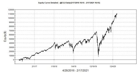
While playing around with this I did some prototyping of a daily bar system and created this equity curve.  I mistakenly did not allow any losses – only took profits and re-entered long.

Wow! Awesome! Holy Grail Uncovered. Venalicius Cave!

Venalicius Cave!  Don’t take a loser you and will reap the benefits.  The chart says so – so its got to be true – I know right?

The same chart from a different perspective.

You Start and End at the Same Place. But What A Ride. Yikes!

Moral of the Story – always look at your detailed Equity Curve.  This curve is very close to a simple buy and hold strategy.   Maybe a little better.

Daily Bar Ratcheting Stop and Conditional Optimization

Happy New Year!  My First Post of 2021!

In this post I simply wanted to convert the intraday ratcheting stop mechanism that I previously posted into a daily bar mechanism.  Well that got me thinking of how many different values could be used as the amount to ratchet.  I came up with three:

I have had requests for the EasyLanguage in an ELD – so here it is – just click on the link and unZip.

RATCHETINGSTOPWSWITCH

Ratcheting Schemes

  • ATR of N days
  • Fixed $ Amount
  • Percentage of Standard Deviation of 20 Days

So this was going to be a great start to a post, because I was going to incorporate one of my favorite programming constructs : Switch-Case.  After doing the program I thought wouldn’t it be really cool to be able to optimize over each scheme the ratchet and trail multiplier as well as the values that might go into each scheme.

In scheme one I wanted to optimize the N days for the ATR calculation.  In scheme two I wanted to optimize the $ amount and the scheme three the percentage of a 20 day standard deviation.  I could do a stepwise optimization and run three independent optimizations – one for each scheme.  Why not just do one global optimization you might ask?  You could but it would be a waste of computer time and then you would have to sift through the results.  Huh?  Why?  Here is a typical optimization loop:

Scheme Ratchet Mult Trigger Mult Parameter 1
1 : ATR 1 1 ATR (2)
2 : $ Amt 1 1 ATR (2)
3 : % of Dev. Amt 1 1 ATR (2)
1 : ATR 2 1 ATR (2)
2 : $ Amt 2 1 ATR (2)

Notice when we switch schemes the Parameter 1 doesn’t make sense.  When we switch to $ Amt we want to use a $ Value as Parameter 1 and not ATR.  So we could do a bunch of optimizations across non sensical values, but that wouldn’t really make a lot of sense.  Why not do a conditional optimization?  In other words, optimize only across a certain parameter range based on which scheme is currently being used.  I knew there wasn’t an overlay available to use using standard EasyLanguage but I thought maybe OOP,  and there is an optimization API that is quite powerful.  The only problem is that it was very complicated and I don’t know if I could get it to work exactly the way I wanted.

EasyLanguage is almost a full blown programming language.  So should I not be able to distill this conditional optimization down to something that I could do with such a powerful programming language?  And the answer is yes and its not that complicated.  Well at least for me it wasn’t but for beginners probably.  But to become a successful programmer you have to step outside your comfort zones, so I am going to not only explain the Switch/Case construct (I have done this in earlier posts)  but incorporate some array stuff.

When performing conditional optimization there are really just a few things you have to predefine:

  1. Scheme Based Optimization Parameters
  2. Exact Same Number of Iterations for each Scheme [starting point and increment value]
  3. Complete Search Space
  4. Total Number of Iterations
  5. Staying inside the bounds of your Search Space

Here are the optimization range per scheme:

  • Scheme #1 – optimize number of days in ATR calculation – starting at 10 days and incrementing by 2 days
  • Scheme #2 – optimize $ amounts – starting at $250 and incrementing by $100
  • Scheme #3 – optimize percent of 20 Bar standard deviation – starting at 0,25 and incrementing by 0.25

I also wanted to optimize the ratchet and target multiplier.  Here is the base code for the daily bar ratcheting system with three different schemes.  Entries are based on penetration of 20 bar highest/lowest close.

inputs: 
ratchetMult(2),trailMult(2),
volBase(True),volCalcLen(20),
dollarBase(False),dollarAmt(250),
devBase(False),devAmt(0.25);


vars:longMult(0),shortMult(0);
vars:ratchetAmt(0),trailAmt(0);
vars:stb(0),sts(0),mp(0);
vars:lep(0),sep(0);


if volBase then
begin
ratchetAmt = avgTrueRange(volCalcLen) * ratchetMult;
trailAmt = avgTrueRange(volCalcLen) * trailMult;
end;
if dollarBase then
begin
ratchetAmt =dollarAmt/bigPointValue * ratchetMult;
trailAmt = dollarAmt/bigPointValue * trailMult;
end;
if devBase then
begin
ratchetAmt = stddev(c,20) * devAmt * ratchetMult;
trailAmt = stddev(c,20) * devAmt * trailMult;
end;


if c crosses over highest(c[1],20) then buy next bar at open;
if c crosses under lowest(c[1],20) then sellshort next bar at open;

mp = marketPosition;
if mp <> 0 and mp[1] <> mp then
begin
longMult = 0;
shortMult = 0;
end;


If mp = 1 then lep = entryPrice;
If mp =-1 then sep = entryPrice;


// Okay initially you want a X point stop and then pull the stop up
// or down once price exceeds a multiple of Y points
// longMult keeps track of the number of Y point multiples of profit
// always key off of lep(LONG ENTRY POINT)
// notice how I used + 1 to determine profit
// and - 1 to determine stop level

If mp = 1 then
Begin
If h >= lep + (longMult + 1) * ratchetAmt then longMult = longMult + 1;
Sell("LongTrail") next bar at (lep + (longMult - 1) * trailAmt) stop;
end;

If mp = -1 then
Begin
If l <= sep - (shortMult + 1) * ratchetAmt then shortMult = shortMult + 1;
buyToCover("ShortTrail") next bar (sep - (shortMult - 1) * trailAmt) stop;
end;
Daily Bar Ratchet System

This code is fairly simple.  The intriguing inputs are:

  • volBase [True of False] and  volCalcLen [numeric Value]
  • dollarBase [True of False] and  dollarAmt [numeric Value]
  • devBase [True of False] and devAmt [numeric Value]

If volBase is true then you use the parameters that go along with that scheme.  The same goes for the other schemes.  So when you run this you would turn one scheme on at a time and set the parameters accordingly.  if I wanted to use dollarBase(True) then I would set the dollarAmt to a $ value.  The ratcheting mechanism is the same as it was in the prior post so I refer you back to that one for further explanation.

So this was a pretty straightforward strategy.  Let us plan out our optimization search space based on the different ranges for each scheme.  Since each scheme uses a different calculation we can’t simply optimize across all of the different ranges – one is days, and the other two are dollars and percentages.

Enumerate

We know how to make TradeStation loop based on the range of a value.  If you want to optimize from $250 to $1000 in steps of $250, you know this involves [$1000 – $250] / $250 + 1 or 3 + 1 or 4 interations.   Four loops will cover this entire search space.  Let’s examine the search space for each scheme:

  • ATR Scheme: start at 10 bars and end at 40 by steps of 2 or [40-10]/2 + 1 = 16
  • $ Amount Scheme: start at $250 and since we have to have 16 iterations [remember # of iterations have to be the same for each scheme] what can we do to use this information?  Well if we start $250 and step by $100 we cover the search space $250, $350, $450, $550…$1,750.  $250 + 15 x 250.  15 because $250 is iteration 1.
  • Percentage StdDev Scheme:  start at 0.25 and end at 0.25 + 15 x 0.25  = 4

So we enumerate 16 iterations to a different value.  The easiest way to do this is to create a map.  I know this seems to be getting hairy but it really isn’t.  The map will be defined as an array with 16 elements.  The array will be filled with the search space based on which scheme is currently being tested.  Take a look at this code where I show how to define an array of 16 elements and introduce my Switch/Case construct.

array: optVals[16](0);

switch(switchMode)
begin
case 1:
startPoint = 10; // vol based
increment = 2;
case 2:
startPoint = 250/bigPointValue; // $ based
increment = 100/bigPointValue;
case 3:
startPoint = 0.25; //standard dev
increment = 0.25*minMove/priceScale;
default:
startPoint = 1;
increment = 1;
end;

vars: cnt(0),loopCnt(0);
once
begin
for cnt = 1 to 16
begin
optVals[cnt] = startPoint + (cnt-1) * increment;
end;
end
Set Up Complete Search Space for all Three Schemes

This code creates a 16 element array, optVals, and assigns 0 to each element.  SwitchMode goes from 1 to 3.

  • if switchMode is 1: ATR scheme [case: 1] the startPoint is set to 10 and increment is set to 2
  • if switchMode is 2: $ Amt scheme [case: 2] the startPoint is set to $250 and increment is set to $100
  • if switchMode is 3: Percentage of StdDev [case: 3] the startPoint is set to 0.25 and the increment is set to 0.25

Once these two values are set the following 15 values can be spawned by the these two.  A for loop is great for populating our search space.  Notice I wrap this code with ONCE – remember ONCE  is only executed at the very beginning of each iteration or run.

once
begin
   for cnt = 1 to 16
   begin
     optVals[cnt] = startPoint + (cnt-1) * increment;
   end;
end

Based on startPoint and increment the entire search space is filled out.  Now all you have to do is extract this information stored in the array based on the iteration number.

Switch(switchMode) 
Begin
Case 1:
ratchetAmt = avgTrueRange(optVals[optLoops]) * ratchetMult;
trailAmt = avgTrueRange(optVals[optLoops]) * trailMult;
Case 2:
ratchetAmt =optVals[optLoops] * ratchetMult;
trailAmt = optVals[optLoops] * trailMult;
Case 3:
ratchetAmt =stddev(c,20) * optVals[optLoops] * ratchetMult;
trailAmt = stddev(c,20) * optVals[optLoops] * trailMult;
Default:
ratchetAmt = avgTrueRange(optVals[optLoops]) * ratchetMult;
trailAmt = avgTrueRange(optVals[optLoops]) * trailMult;
end;


if c crosses over highest(c[1],20) then buy next bar at open;
if c crosses under lowest(c[1],20) then sellshort next bar at open;

mp = marketPosition;
if mp <> 0 and mp[1] <> mp then
begin
longMult = 0;
shortMult = 0;
end;


If mp = 1 then lep = entryPrice;
If mp =-1 then sep = entryPrice;


// Okay initially you want a X point stop and then pull the stop up
// or down once price exceeds a multiple of Y points
// longMult keeps track of the number of Y point multiples of profit
// always key off of lep(LONG ENTRY POINT)
// notice how I used + 1 to determine profit
// and - 1 to determine stop level

If mp = 1 then
Begin
If h >= lep + (longMult + 1) * ratchetAmt then longMult = longMult + 1;
Sell("LongTrail") next bar at (lep + (longMult - 1) * trailAmt) stop;
end;

If mp = -1 then
Begin
If l <= sep - (shortMult + 1) * ratchetAmt then shortMult = shortMult + 1;
buyToCover("ShortTrail") next bar (sep - (shortMult - 1) * trailAmt) stop;
end;
Extract Search Space Values and Rest of Code

Switch(switchMode)
Begin
Case 1:
  ratchetAmt = avgTrueRange(optVals[optLoops])ratchetMult;
  trailAmt = avgTrueRange(optVals[optLoops]) trailMult;
Case 2:
  ratchetAmt =optVals[optLoops] * ratchetMult;
  trailAmt = optVals[optLoops] * trailMult;
Case 3:
  ratchetAmt =stddev(c,20)optVals[optLoops]
ratchetMult;
  trailAmt = stddev(c,20) * optVals[optLoops] * trailMult;

Notice how the optVals are indexed by optLoops.  So the only variable that is optimized is the optLoops and it spans 1 through 16.  This is the power of enumerations – each number represents a different thing and this is how you can control which variables are optimized in terms of another optimized variable.   Here is my optimization specifications:

Opimization space

And here are the results:

Optimization Results

The best combination was scheme 1 [N-day ATR Calculation] using a 2 Mult Ratchet and 1 Mult Trail Trigger.  The best N-day was optVals[2] for this scheme.  What in the world is this value?  Well you will need to back engineer a little bit here.  The starting point for this scheme was 10 and the increment was 2 so if optVals[1] =10 then optVals[2] = 12 or ATR(12).    You can also print out a map of the search spaces.

vars: cnt(0),loopCnt(0);
once
begin
loopCnt = loopCnt + 1;
// print(switchMode," : ",d," ",startPoint);
// print(" ",loopCnt:2:0," --------------------");
for cnt = 1 to 16
begin
optVals[cnt] = startPoint + (cnt-1) * increment;
// print(cnt," ",optVals[cnt]," ",cnt-1);
end;
end;
  Scheme 1
--------------------
1.00 10.00 0.00 10 days
2.00 12.00 1.00
3.00 14.00 2.00
4.00 16.00 3.00
5.00 18.00 4.00
6.00 20.00 5.00
7.00 22.00 6.00
8.00 24.00 7.00
9.00 26.00 8.00
10.00 28.00 9.00
11.00 30.00 10.00
12.00 32.00 11.00
13.00 34.00 12.00
14.00 36.00 13.00
15.00 38.00 14.00
16.00 40.00 15.00

Scheme2
--------------------
1.00 5.00 0.00 $ 250
2.00 7.00 1.00 $ 350
3.00 9.00 2.00 $ 400
4.00 11.00 3.00 $ ---
5.00 13.00 4.00
6.00 15.00 5.00
7.00 17.00 6.00
8.00 19.00 7.00
9.00 21.00 8.00
10.00 23.00 9.00
11.00 25.00 10.00
12.00 27.00 11.00
13.00 29.00 12.00
14.00 31.00 13.00
15.00 33.00 14.00
16.00 35.00 15.00 $1750

Scheme 3
--------------------
1.00 0.25 0.00 25 % stdDev
2.00 0.50 1.00
3.00 0.75 2.00
4.00 1.00 3.00
5.00 1.25 4.00
6.00 1.50 5.00
7.00 1.75 6.00
8.00 2.00 7.00
9.00 2.25 8.00
10.00 2.50 9.00
11.00 2.75 10.00
12.00 3.00 11.00
13.00 3.25 12.00
14.00 3.50 13.00
15.00 3.75 14.00
16.00 4.00 15.00

This was a elaborate post so please email me with questions.  I wanted to demonstrate that we can accomplish very sophisticated things with just the pure and raw EasyLanguage which is a programming language itself.

A Simple Break Out Algorithm Demonstrating Time Optimization

What is Better:  30, 60, or 120 Minute Break-Out on ES.D

Here is a simple tutorial you can use as a foundation to build a potentially profitable day trading system.  Here we wait N minutes after the open and then buy the high of the day or short the low of the day and apply a protective stop and profit objective.  The time increment can be optimized to see what time frame is best to use.  You can also optimize the stop loss and profit objective – this system gets out at the end of the day.  This system can be applied to any .D data stream in TradeStation or Multicharts.

Logic Description

  1. get open time
  2. get close time
  3. get N time increment
    1. 15 – first 15 minute of day
    2. 30 – first 30 minute of day
    3. 60 – first hour of day
  4. get High and Low of day
  5. place stop orders at high and low of day – no entries late in day
  6. calculate buy and short entries – only allow one each*
  7. apply stop loss
  8. apply profit objective
  9. get out at end of day if not exits have occurred

Optimization Results [From 15 to 120 by 5 minutes] on @ES.D 5 Minute Chart – Over Last Two Years

Optimization of Time: Look How the # Trades Decrease as the Time Increment Increases

Simple Orbo EasyLanguage

I threw this together rather quickly in a response to a reader’s question.  Let me know if you see a bug or two.  Remember once you gather your stops you must allow the order to be issued on every subsequent bar of the trading day.  The trading day is defined to be the time between timeIncrement and endTradeMinB4Close.  Notice how I used the EL function calcTime to calculate time using either a +positive or -negative input.  I want to sample the high/low of the day at timeIncrement and want to trade up until endTradeMinB4Close time.  I use the HighD and LowD functions to extract the high and low of the day up to that point.  Since I am using a tight stop relative to today’s volatility you will see more than 1 buy or 1 short occurring.  This happens when entry/exit occurs on the same bar and MP is not updated accordingly.  Somewhere  hidden in this tome of a blog you will see a solution for this.  If you don’t want to search I will repost it tomorrow.


//Optimizing Time to determine a simple break out
//Only works on .D data streams
Inputs: timeIncrement(15),endTradeMinB4Close(-15),stopLoss$(500),profTarg$(1000);

vars: firstBarTime(0),lastBarTime(0),buyStop(0),shortStop(0),
calcStopTime(0),quitTradeTime(0),buysToday(0),shortsToday(0),mp(0);

firstBarTime = sessionStartTime(0,1);
lastBarTime = sessionEndTime(0,1);

calcStopTime = calcTime(firstBarTime,timeIncrement);
quitTradeTime = calcTime(lastBarTime,endTradeMinB4Close);


If time = calcStopTime then
begin
buyStop = HighD(0);
shortStop = LowD(0);
buysToday = 0;
shortsToday = 0;
End;

if time >= calcStopTime and time < quitTradeTime then
begin
if buysToday = 0 then Buy next bar at buyStop stop;
if shortsToday = 0 then Sell short next bar at shortStop stop;
end;

mp = marketPosition;

If mp = 1 then buysToday = 1;
If mp = -1 then shortsToday = 1;

SetStopLoss(stopLoss$);
setProfitTarget(profTarg$);
setExitOnClose;
Orbo EasyLanguage Code