AI can write structure, but experienced programmers still supply the craft
The more we rely on generated code, the more disciplined we must become in questioning it.
AI and modern frameworks now provide valuable insights that, just a few years ago, would have required significant time and effort to obtain. However, while they offer tremendous macro-level leverage, they can also introduce subtle assumptions that lead to impossible scenarios and misleading downstream analysis. This is especially true in environments designed for rapid idea testing, where convenience can come at the expense of deeper, microscopic introspection.
For example, in my PatternSmasher framework, I use constructs like BarsSinceEntry to control trade duration and evaluate pattern efficacy. This makes it very easy to test thousands of ideas quickly. But that convenience comes with a responsibility. If you rely on these abstractions without thinking through the details, you can end up with behavior that looks perfectly valid in code but could never occur in the real world.
I have seen this problem in other frameworks and in AI-generated code as well. This is why it is so important to continue to hone your craft and take a deep dive into the results produced by generated code. In the quant world, the first step is to study the trades and isolate problems such as what I call simultaneous same-direction exit and reentry. Once you see it, the job is to fix it without changing the intent of the algorithm.
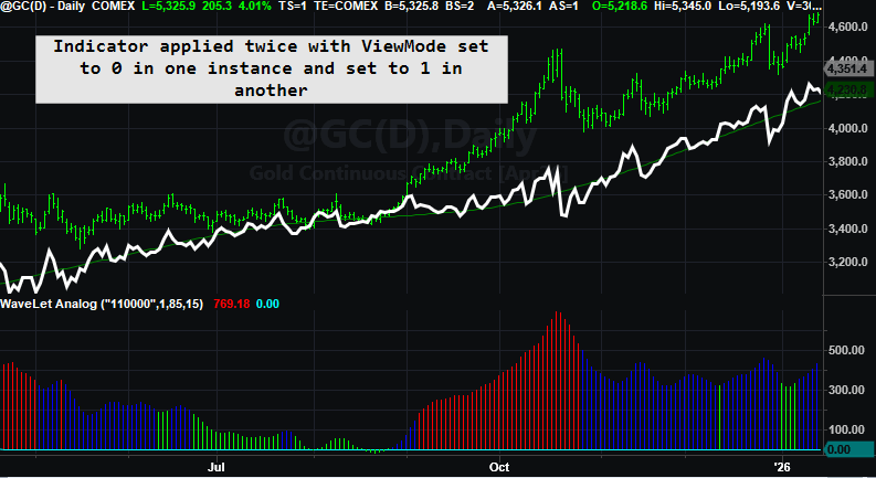
Let me show you exactly what I mean. The logic behind this example looks perfectly fine on the surface. But when you dig into the trades, you see the problem immediately. In this chart, the system exits a long position and then turns right around and buys again at the same time and price. That is not a reversal. It is a same direction exit and reentry that simply cannot happen in the real world, and it pollutes the back test with trades that should not exist.

We entered a long position, the trade expired, immediately re-entered on the next setup, that trade expired as well, and then entered again—only to get stopped out. That’s three round turns, each incurring commission and slippage.
The code that produced this looks pretty clean. You have your entry logic, a BarsSinceEntry exit, and a stop loss. On the surface, everything seems fine.
But you don’t find this kind of problem by staring at the code. You find it by looking at the trades. This is the one thing AI or a framework doesn’t examine. At first, the natural reaction is to slap a MarketPosition “gate” on the entry logic. The word “gate” may be a dead giveaway that AI has influenced the discussion. But I like it. It has been around since the early days of electrical circuits, and it is very appropriate here. I’ve noticed that many of the words AI uses have started to creep into my own vocabulary. Funny how that happens.
Fix #1
So what does that MarketPosition “gate” actually do?
It fixes the symptom. The same-bar exit and reentry disappears, and the trades look cleaner.
But it also changes the algorithm in a much deeper way.
In the original design, a new long signal while already long reaffirmed the position and should have kept the trade alive. The gate removes that behavior. Now the strategy must exit first and then wait until the next bar to reenter.
And that delay matters.
By the time the next bar arrives, the setup may be gone. What should have been one continuous trade is now split into pieces—or missed entirely.
You didn’t just clean up the trades. You changed which trades exist. The new strategy more or may not be more efficient, but just know the algorithm is now different.
Fix #2

We bought, suppressed the expiration exit due to a new buy setup—twice—and were ultimately stopped out at the level where the stop loss from the final trade that didn’t occur—but whose properties we were monitoring—would have been triggered.
Could most quants who aren’t programmers solve this riddle? Probably not. My 40 years of programming experience certainly played a role, and my familiarity with EasyLanguage—especially its limitations—helped guide me down the right path. But more importantly, I was able to recognize the nature of the problem, apply targeted fixes, and then analyze the resulting trades. I repeated this process—wash, rinse, repeat—until the issue was resolved.
Much of the knowledge I relied on has been documented by myself and others over the years. Investing time in books, videos, and webcasts specific to your programming language remains essential—it forms the foundation. But ultimately, refining your own skills and developing your craft is a time-consuming process that pays lasting dividends.
Groundwork for the Fix
Solving what initially appears to be a simple riddle requires recognizing several underlying behaviors. I was able to correct the issue because I could anticipate when a new trade was about to occur. When both the exit gate for an existing position and the entry gate for a new position in the same direction were simultaneously open, I prevented the transition by closing both gates.
However, simply blocking the transition was not enough. I had to simulate the trade that would have occurred. This meant marking the hypothetical entry price, resetting the stop-loss based on that price, and reinitializing my own bars-in-trade counter.
At this point, I could no longer rely on EasyLanguage’s built-in functions such as BarsSinceEntry or SetStopLoss. Those functions assume an actual executed trade and therefore could not reflect the internal state I needed to maintain. To solve the problem correctly, I had to take full control of trade state management and explicitly track these values myself.
This version fixes the problem by taking control of the trade state instead of relying on EasyLanguage’s built-in functions.
First, I define whether I can go long or short, independent of my current position. Then I track my own state variables—market position, bars in trade, stop levels, and trade count—so I know exactly what the system is doing at all times.
The key occurs when a same-direction signal appears after the trade has technically expired. Instead of allowing an exit and immediate reentry, I suppress both actions and simulate the renewed trade. I mark the hypothetical entry price, reset the stop based on that level, and restart my bars-in-trade counter.
Because of this, I can no longer rely on BarsSinceEntry or SetStopLoss—they depend on actual trades. I manage everything explicitly.
The result is a continuous position that preserves the original intent of the algorithm without introducing impossible trades into the backtest.
EasyLanguage also has its share of esoteric nuances. Code order can matter in some places and not in others, particularly with order execution. Even detecting position changes requires a bit of finesse. These details matter, but they are beyond the scope of this discussion.
This is where the difference between generated code and engineered code becomes clear.
A programmer who is not willing to put in the work—and instead relies on AI to solve the problem—will likely stop at the first acceptable fix. The code will run, the trades will look cleaner, and the issue will appear resolved. But the deeper problem remains: the structure has changed, trades may be missing, and the original intent of the algorithm has been compromised.
As we become more dependent on code generation through AI and frameworks, it becomes even more important to validate that the output is reasonable and reflects something that could occur in the real world. That responsibility does not go away—it increases. And it requires us to continue honing our craft.
AI can generate code and even suggest reasonable fixes, but it does not truly understand the nuances of the language, the sequencing of events, or the intent behind the strategy. It cannot look at a trade and say, “that shouldn’t have happened.” It does not debug by questioning reality—it follows patterns.
Arriving at the correct solution required recognizing the problem, iterating through possible fixes, examining the trades, and refining the logic until the behavior matched the intent. That process—wash, rinse, repeat—is the craft.
Generated code can get you started. Engineered code is what gets you to the truth. Take a look at the two following reports. Similar results, but look at the number of trades and those statistics tied to this number.