Well it’s been a year, this month, that Murray passed away. I was fortunate to work with him on many of his projects and learned quite a bit about inter-market convergence and divergence. Honestly, I wasn’t that into it, but you couldn’t argue with his results. A strategy that he developed in the 1990s that compared the Bond market with silver really did stand the test of time. He monitored this relationship over the years and watched in wane. Murray replaced silver with $UTY.
The PHLX Utility Sector Index (UTY) is a market capitalization-weighted index composed of geographically diverse public utility stocks.
He wrote an article for EasyLanguage Mastery by Jeff Swanson where he discussed this relationship and the development of inter-market strategies and through statistical analysis proved that these relationships added real value.
I am currently writing Advanced Topics, the final book in my Easing Into EasyLanguage trilogy, and have been working with Murray’s research. I am fortunate to have a complete collection of his Futures Magazine articles from the mid 1990s to the mid 2000s. There is a quite a bit of inter-market stuff in his articles. I wanted, as a tribute and to proffer up some neat code, to show the performance and code of his Bond and $UTY inter-market algorithm.
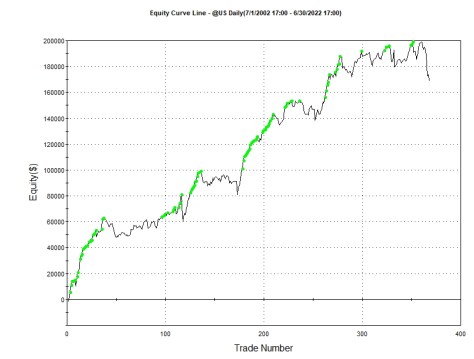
Here is a version that he published a few years ago updated through June 30, 2022 – no commission/slippage.
Not a bad equity curve. To be fair to Murray he did notice the connection between $UTY and the bonds was changing over the past couple of year. And this simple stop and reverse system doesn’t have a protective stop. But it wouldn’t look much different with one, because the system looks at momentum of the primary data and momentum of the secondary data and if they are in synch (either positively or negatively correlated – selected by the algo) an order is fired off. If you simply just add a protective stop, and the momentum of the data are in synch, the strategy will just re-enter on the next bar. However, the equity curve just made a new high recently. It has got on the wrong side of the Fed raising rates. One could argue that this invisible hand has toppled the apple cart and this inter-market relationship has been rendered meaningless.
Murray had evolved his inter-market analysis to include state transitions. He not only looked at the current momentum, but also at where the momentum had been. He assigned the transitions of the momentum for the primary and secondary markets a value from one to four and he felt this state transition helped overcome some of the coupling/decoupling of the inter-market relationship.
However, I wanted to test Murray’s simple strategy with a fixed $ stop and force the primary market to move from positive to negative or negative to positive territory while the secondary market is in the correct relationship. Here is an updated equity curve.
This equity curve was developed by using a $4500 stop loss. Because I changed the order triggers, I reoptimized the length of the momentum calculations for the primary and secondary markets. This curve is only better in the category of maximum draw down. Shouldn’t we give Murray a chance and reoptimize his momentum length calculations too! You bet.
These metrics were sorted by Max Intraday Draw down. The numbers did improve, but look at the Max Losing Trade value. Murray’s later technology, his State Systems, were a great improvement over this basic system. Here is my optimization using a slightly different entry technique and a $4500 protective stop.
This system, using Murray’s overall research, achieved a better Max Draw Down and a much better Max Losing Trade. Here is my code using the template that Murray provided in his articles in Futures Magazine and EasyLanguage Mastery.
// Code by Murray Ruggiero // adapted by George Pruitt
If Type=0 Then Begin InterInd=Close of Data(InterSet)-CLose[LenInt] of Data(InterSet); MarkInd=CLose-CLose[LenTr]; end;
If Type=1 Then Begin InterInd=Close of Data(InterSet)-Average(CLose of Data(InterSet),LenInt); MarkInd=CLose-Average(CLose,LenTr); end;
if Relate=1 then begin If InterInd > 0 and MarkInd CROSSES BELOW 0 and LSB>=0 then Buy("GO--Long") Next Bar at open; If InterInd < 0 and MarkInd CROSSES ABOVE 0 and LSB<=0 then Sell Short("GO--Shrt") Next Bar at open;
end; if Relate=0 then begin If InterInd<0 and MarkInd CROSSES BELOW 0 and LSB>=0 then Buy Next Bar at open; If InterInd>0 and MarkInd CROSSES ABOVE 0 and LSB<=0 then Sell Short Next Bar at open; end;
Here the user can actually include more than two data streams on the chart. The InterSet input allows the user to choose or optimize the secondary market data stream. Momentum is defined by two types:
Type 0: Intermarket or secondary momentum simply calculated by close of data(2) – close[LenInt] of date(2) and primary momentum calculated by close – close[LenTr]
Type 1: Intermarket or secondary momentum calculated by close of data(2) – average( close of data2, LenInt) and primary momentum calculated by close – average(close, LenTr)
The user can also input what type of Relationship: 1 for positive correlation and 0 for negative correlation. This template can be used to dig deeper into other market relationships.
George’s Modification
I simply forced the primary market to CROSS below/above 0 to initiate a new trade as long the secondary market was pointing in the right direction.
If InterInd > 0 and MarkInd CROSSES BELOW 0 and LSB>=0 then Buy("GO--Long") Next Bar at open; If InterInd < 0 and MarkInd CROSSES ABOVE 0 and LSB<=0 then Sell Short("GO--Shrt") Next Bar at open;
Using the keyword CROSSES
This was a one STATE transition and also allowed a protective stop to be used without the strategy automatically re-entering the trade in the same direction.
Thank You Murray – we sure do miss you!
Murray loved to share his research and would want us to carry on with it. I will write one or two blogs a year in tribute to Murray and his invaluable research.
Quickly Analyze Market Metrics with Gradient Based Shading
This is a simple indicator but it does involve some semi-advanced topics. Just to let you know I am working on the third book in the Easing Into EasyLanguage series. If you haven’t check out the first two, you might just want to head over to amazon and check those out. This topic falls in the spectrum of the ideas that I will be covering in the Advanced Topics edition. Also to let you know I just published the 2nd Edition of Trend Following Systems: A DIY Project – Batteries Included. Check this out if you want to learn some Python and also see some pretty cool Trend Following algorithms – I include EasyLanguage too!
The code that follows demonstrates how to shade between plots and adjust gradient in terms of the RSI reading. I compiled this with MultiCharts, so I assume it will work there too – just let me know if it doesnt. I found this code somewhere on the web when researching shading. If I knew the original author I would definitely give full credit. The code is rather simple, setting up the chart is just slightly more difficult. The Keltner Channel was used to define the shading boundaries. You could have just as easily used Bollinger Bands or anything that provided a range around the market. Here’s the code.
Basically all this math is doing is keeping the RSI reading within the bounds of the Keltner Upper and Lower Channels. You want a high RSI reading to be near the Upper Channel and a low RSI reading to be near the Lower Channel. You can change up the formula to make more sense.
I have worked with computer graphics for many years and this is really a very neat formula. The generic formula to constrain a value within a boundary is;
Here you take the LowerBand and add the percentage of the MyRSI/100 times the range. This works too. But the original formula scales or intensifies the RSI reading so you get much wider gradient spectrum. The AVG is used as the center of gravity and the RSI is converted in terms of the middle 50 line. A positive number, anything > 50, is then scaled higher in the range and a negative number, anything < 50 is scaled lower in the range. In other words it makes a prettier and more informative picture.
Returns a specific color from a user defined gradient color range, such as Blue to White
Inputs:
dValue = value being passed-in that is within the specified Min/Max range of values
dMin = Starting value for the gradient range, where the nFromColor is displayed
dMax = Ending value for the gradient range, where the nToColor is displayed
nFromColor = Starting color of the gradient
nToColor = Ending color of the gradient
Since the gradient shading will cover up your bars you will need to plot the bars as well.
Chart SetUp
Don’t Forget To Fade Out Your Data Chart
That’s it. Like I stated earlier – I will be including things like this in the Advanced Topics edition. I should have it wrapped sometime in July or August.
Sometimes you just want to create a combined equity curve of several markets and for one reason or another you don’t want to use Maestro. This post will show you an indicator that you can insert into your TradeStation chart/strategies that will output monthly cumulative equity readings. After that I refresh my VBA skills a little bit by creating a VBA Macro/Script that will take the output and parse it into a table where the different months are the rows and the different market EOM equities, for those months, will be the columns. Then all the rows will be summed and then finally a chart will be produced. I will zip the Exel .xlsm and include it at the end of this post.
Part 1: Output Monthly Data to Print Log
You can determine the end of the month by comparing the current month of the date and the month of the prior date. If they are different, then you know you are sitting on the first trading day of the new month. You can then reach back and access the total equity as of yesterday. If you want you can also track the change in month equity. Here is the indicator code in EasyLanguage.
// Non plotting indicator that needs to be applied to // a chart that also has a strategy applied // one that produces a number of trades
if month(date) <> month(date[1]) then begin monthlyEqu = totalEquity[1] - priorMonthEqu; priorMonthEqu = totalEquity[1]; print(getSymbolName,",",month(date[1]):2:0,"-",year(date[1])+1900:4:0,",",monthlyEqu,",",totalEquity); end; totalEquity = i_ClosedEquity;
Indicator that exports the EOM equity values
The interesting part of this code is the print statement. You can use the month and year functions to extract the respective values from the date bar array. I use a formatted print to export the month and year without decimals. Remember 2021 in TradeStation is represented by 121 and all you have to do is add 1900 to get a more comfortable value. The month output is formatted with :2:0 and the year with :4:0. The first value in the format notation informs the computer to allow at least 2 or 4 values for the month and the year respectively. The second value following the second colon informs the computer that you do not want any decimals values (:0). Next insert the indicator into all the charts in your workspace. Here’s a snippet of the output on one market. I tested this on six markets and this data was the output generated. Some of the markets were interspersed and that is okay. You may have a few months of @EC and then a few months of @JY and then @EC again.
If you use this post’s EXCEL workbook with the macro you may need to tell EXCEL to forget any formatting that might already be inside the workbook. Open my workbook and beware that it will inform/warn you that a macro is located inside and that it could be dangerous. If you want to go ahead and enable the macro go ahead. On Sheet1 click in A1 and place the letter “G”. Then goto the Data Menu and then the Data Tools section of the ribbon and click Text to Columns. A dialog will open and ask you they type of file that best describes your data. Click the Delimited radio button and then next. You should see a dialog like this one.
Now copy all of the data from the Print-Log and paste it into Column A. If all goes right everything will be dumped in the appropriate rows and in a single column.
First select column A and go back to the Data Menu and the Data Tools on the Ribbon. Select Delimited and hit next, Choose comma because we used commas to separate our values. Click Next again. Eventually you will get to this dialog.
If you chose Date format for column 2 with MDY, then it will be imported into the appropriate column in a date format. This makes charting easier. If all goes well then you will have four columns of data – a column for Symbol, Date, Delta-EOM and EOM. Select column B and right click and select Format Cells.
Once you format the B column in the form of MM-YYYY you will have a date like 9-2007, 10-2007, 11-2007…
Running the VBA Macro/Script
On the Ribbon in EXCEL goto the Developer Tab. If you don’t see it then you will need to install it. Just GOOGLE it and follow their instructions. Once on the Develop Tab goto the Code category and click the Visual Basic Icon. Your VBA IDE will open and should like very similar to this.
If all goes according to plan after you hit the green Arrow for the Run command your spreadsheet should like similar to this.
The Date column will be needed to be reformatted again as Date with Custom MM-YYYY format. Now copy the table by highlighting the columns and rows including the headings and then goto to Insert Menu and select the Charts category.
This is what you should get.
This is the output of the SuperTurtle Trading system tested on the currency sector from 2007 to the present.
VBA Code
I have become very spoiled using Python as it does many things for you by simply calling a function. This code took my longer to develop than I thought it would, because I had to back to the really old school of programming (really wanted to see if I could do this from scratch) to get this done. You could of course eliminate some of my code by calling spread sheet functions from within EXCEL. I went ahead and did it the brute force way just to see if I could do it.
Sub combineEquityFromTS()
'read data from columns 'symbol, date, monthlyEquity, cumulativeEquity - format 'create arrays to hold each column of data 'use nested loops to do all the work 'brute force coding, no objects - just like we did in the 80s
Dim symbol(1250) As String Dim symbolHeadings(20) As String Dim myDate(1250) As Long Dim monthlyEquity(1250) As Double Dim cumulativeEquity(1250) As Double
'read the data from the cells dataCnt = 1 Do While Cells(dataCnt, 1) <> "" symbol(dataCnt) = Cells(dataCnt, 1) myDate(dataCnt) = Cells(dataCnt, 2) monthlyEquity(dataCnt) = Cells(dataCnt, 3) cumulativeEquity(dataCnt) = Cells(dataCnt, 4) dataCnt = dataCnt + 1 Loop dataCnt = dataCnt - 1
'get distinct symbolNames and use as headers symbolHeadings(1) = symbol(1) numSymbolheadings = 1 For i = 2 To dataCnt - 1 If symbol(i) <> symbol(i + 1) Then newSymbol = True For j = 1 To numSymbolheadings If symbol(i + 1) = symbolHeadings(j) Then newSymbol = False End If Next j If newSymbol = True Then numSymbolheadings = numSymbolheadings + 1 symbolHeadings(numSymbolheadings) = symbol(i + 1) End If End If Next i
'Remove duplicate months in date array 'have just one column of month end dates
Cells(2, 7) = myDate(1) dispRow = 2 numMonths = 1 i = 1 Do While i <= dataCnt foundDate = False For j = 1 To numMonths If myDate(i) = Cells(j + 1, 7) Then foundDate = True End If Next j If foundDate = False Then numMonths = numMonths + 1 Cells(numMonths + 1, 7) = myDate(i) End If i = i + 1 Loop 'put symbols across top of table 'put "date" and "cumulative" column headings in proper 'locations too
Cells(1, 7) = "Date" For i = 1 To numSymbolheadings Cells(1, 7 + i) = symbolHeadings(i) Next i
numSymbols = numSymbolheadings Cells(1, 7 + numSymbols + 1) = "Cumulative" 'now distribute the monthly returns in their proper 'slots in the table dispRow = 2 dispCol = 7 For i = 1 To numSymbols For j = 2 To numMonths + 1 For k = 1 To dataCnt foundDate = False If symbol(k) = symbolHeadings(i) And myDate(k) = Cells(j, 7) Then Cells(dispRow, dispCol + i) = cumulativeEquity(k) dispRow = dispRow + 1 Exit For End If 'for later use 'If j > 1 Then ' If symbol(k) = symbolHeadings(i) And myDate(k) < Cells(j, 7) And myDate(k) > Cells(j - 1, 7) Then ' dispRow = dispRow + 1 ' End If 'End If Next k Next j dispRow = 2 Next i 'now accumulate across table and then down For i = 1 To numMonths cumulative = 0 For j = 1 To numSymbols cumulative = cumulative + Cells(i + 1, j + 7) Next j Cells(i + 1, 7 + numSymbols + 1) = cumulative Next i End Sub
This a throwback to the 80s BASIC on many of the family computers of that era. If you are new to VBA you can access cell values by using the keyword Cells and the row and column that points to the data. The first thing you do is create a Module named combineEquityFromTS and in doing so it will create a Sub combineEquityFromTS() header and a End Sub footer. All of your code will be squeezed between these two statements. This code is ad hoc because I just sat down and started coding without much forethought.
Use DIM to Dimension an Arrays
I like to read the date from the cells into arrays so I can manipulate the data internally. Here I create five arrays and then loop through column one until there is no longer any data. The appropriate arrays are filled with their respective data from each row.
Once the data is in arrays we can start do parse it. The first thing I want is to get the symbolHeadings or markets. I know the first row has a symbol name so I go ahead and put that into the symbolHeadings array. I kept track of the number of rows in the data with the variable dataCnt. Here I use nested loops to work my way down the data and keep track of new symbols as I encounter them. If the symbol changes values, I then check my list of stored symbolHeadings and if the new symbol is not in the list I add it.
Since all the currencies will have the same month values I wanted to compress all the months into a single discrete month list. This isn’t really all that necessary since we could have just prefilled the worksheet with monthly date values going back to 2007. This algorithm is similar to the one that is used to extract the different symbols. Except this time, just for giggles, I used a Do While Loop.
As well as getting values from cells you can also put values into them. Here I run through the list of markets and put them into Cells(1, 7+i). When working with cells you need to make sure you get the offset correct. Here I wanted to put the market names in Row A and Columns: H, I, J, K, L, M.
Column H = 8
Column I = 9
Column J = 10
Column K =11
Column L = 12
Column M = 13
Cells are two dimensional arrays. However if you are going to use what is on the worksheet make sure you are referencing the correct data. Here I introduce dispRow and dispCol as the anchor points where the data I need to reference starts out.
Here I first parse through each symbol and extract the EOM value that matches the symbol name and month-year value. So if I am working on @EC and I need the EOM for 07-2010, I fist loop through the month date values and compare the symbol AND myDate (looped through with another for-loop) with the month date values. If they are the same then I dump the value in the array on to the spreadsheet. And yes I should have used this:
For j = dispRow to numMonths-1
Instead of –
For j = 2 to numMonths-1
Keeping arrays in alignment with Cells can be difficult. I have a hybrid approach here. I will clean this up later and stick just with arrays and only use Cells to extract and place data. The last thing you need to do is sum each row up and store that value in the Cumulative column.
Conclusion
This was another post where we relied on another application to help us achieve our objective. If you are new to EXCEL VBA (working with algorithms that generate trades) you can find out more in my Ultimate Algorithmic Trading System Toolbox book. Even if you don’t get the book this post should get you started on the right track.
SuperTrend is a trading strategy and indicator all built into one entity. There are a couple of versions floating around out there. MultiCharts and Sierra Chart both have slightly different flavors of this combo approach.
Ratcheting Trailing Stop Paradigm
This indic/strat falls into this category of algorithm. The indicator never moves away from your current position like a parabolic stop or chandelier exit. I used the code that was disclosed on Futures.io or formerly known as BigMikesTrading blog. This version differs from the original SuperTrend which used average true range. I like Big Mike’s version so it will discussed here.
Big Mike’s Math
The math for this indicator utilizes volatility in the terms of the distance the market has travelled over the past N days. This is determined by calculating the highest high of the last N days/bars and then subtracting the lowest low of last Ndays/bars. Let’s call this the highLowRange. The next calculation is an exponential moving average of the highLowRange. This value will define the market volatility. Exponential moving averages of the last strength days/bars highs and lows are then calculated and divided by two – giving a midpoint. The volatility measure (multiplied my mult) is then added to this midpoint to calculate an upper band. A lower band is formed by subtracting the volatility measure X mult from the midpoint.
Upper or Lower Channel?
If the closing price penetrates the upper channel and the close is also above the highest high of strength days/bars back (offset by one of course) then the trend will flip to UP. When the trend is UP, then the Lower Channel is plotted. Once the trend flips to DN, the upper channel will be plotted. If the trend is UP the lower channel will either rise with the market or stay put. The same goes for a DN trend – hence the ratcheting. Here is a graphic of the indicator on CL.
If you plan on using an customized indicator in a strategy it is always best to build the calculations inside a function. The function then can be used in either an indicator or a strategy.
Function Name: SuperTrend_BM
Function Type: Series – we will need to access prior variable values
if trend < 0 and trend[1] > 0 then trendDN = True; if trend > 0 and trend[1] < 0 then trendUP = True;
//ratcheting mechanism if trend > 0 then dn = maxList(dn,dn[1]); if trend < 0 then up = minList(up,up[1]);
// if trend dir. changes then assign // up and down appropriately if trendUP then up = xAvg + mult * xAvgRng; if trendDN then dn = xAvg - mult * xAvgRng;
if trend = 1 then ST = dn else ST = up;
STrend = trend;
SuperTrend_BM = ST;
SuperTrend ala Big Mike
The Inputs to the Function
The original SuperTrend did include the Strength input. This input is a Donchian like signal. Not only does the price need to close above/below the upper/lower channel but also the close must be above/below the appropriate Donchian Channels to flip the trend, Also notice we are using a numericRef as the type for STrend. This is done because we need the function to return two values: trend direction and the upper or lower channel value. The appropriate channel value is assigned to the function name and STrend contains the Trend Direction.
A Function Driver in the Form of an Indicator
A function is a sub-program and must be called to be utilized. Here is the indicator code that will plot the values of the function using: length(9), mult(1), strength(9).
// SuperTrend indicator // March 25 2010 // Big Mike https://www.bigmiketrading.com inputs: length(9), mult(1), strength(9);
vars: strend(0), st(0);
st = SuperTrend_BM(length, mult,strength,strend);
if strend = 1 then Plot1(st,"SuperTrendUP"); if strend = -1 then Plot2(st,"SuperTrendDN");
Function Drive in the form of an Indicator
This should be a fun indicator to play with in the development of a trend following approach. My version of Big Mike’s code is a little different as I wanted the variable names to be a little more descriptive.
Update Feb 28 2022
I forgot to mention that you will need to make sure your plot lines don’t automatically connect.
Can You Do This with Just One Plot1?
An astute reader brought it to my attention that we could get away with a single plot and he was right. The reason I initially used two plot was to enable the user to chose his/her own plot colors by using the Format dialog.
//if strend = 1 then Plot1(st,"SuperTrendUP"); //if strend = -1 then Plot2(st,"SuperTrendDN");
if strend = 1 then SetPlotColor(1,red); if strend = -1 then SetPlotColor(1,green);
In writing the Hi-Res edition of Easing Into EasyLanguage I should have included this sample program. I do point out the limitations of the EntryPrice keyword/function in the book. But recently I was tasked to create a pyramiding scheme template that used minute bars and would initiate a position with N Shares and then pyramid up to three times by adding on N Shares at the last entry price + one 10 -Day ATR measure as the market moves in favor of the original position. Here is an example of just such a trade.
EntryPrice only contains the original entry price. So every time you add on a position, the EntryPrice doesn’t reflect this add on price. I would like to be able to index into this keyword/function and extract any EntryPrice. If you enter at the market, then you can keep track of entry prices because a market order is usually issued from an if-then construct:
//Here I can keep track of entry prices because I know //exactly when and where they occur.
if c > c[1] and value1 > value2 then begin buy("MarketOrder") next bar at market; lastEntryPrice = open of next bar; end;
Last Entry Price tracking is easy if using Market Orders
But what if you are using a stop or limit order. You don’t know ahead of time where one of these types of orders will hit up. It could be the next bar or it could be five bars later or who knows.
AvgEntryPrice Makes Up for the Weakness of EntryPrice
AvgEntryPrice is a keyword/function that returns the average of the entries when pyramiding. Assume you buy at 42.00 and pyramid the same number of shares at 46.50 – AvgEntryPrice will be equal to (42.00 + 46.50) / 2 = 44.25. With this information you can determine the two entry prices. You already know the original price. Take a look at this code.
// remember currentShares and avgEntryPrice ARE EasyLanguage Keywords/Functions if mp[1] = mp and mp = -1 and currentShares > curShares then begin totShorts = totShorts + 1; if currentShares > initShares then begin lastEntryPrice = totShorts * avgEntryPrice - entryPriceSums; entryPriceSums = entryPriceSums + lastEntryPrice; print(d," Short addon ",lastEntryPrice," ",totShorts," ",avgEntryPrice," ",entryPriceSums); end; end;
Calculating the true LastEntryPrice
Remember currentShares is a keyword/function and it is immediately updated when more shares are added or taken off. CurShares is my own variable where I keep track of the prior currentShares , so if currentShares (real number of shares) is greater than the prior curShares (currentShares) then I know 100%, a position has been pyramided as long the the mp stays the same. If currentShares increases and mp stays constant, then you can figure out the last entry price where the pyramid takes place. First you tick totShorts up by 1. If currentShares > initShares, then you know you are pyramiding so
Don’t believe me. Let’s test it. Remember original entry was 42.00 and the add on was at 46.50. TotShorts now equals 2.
Initial entryPrice = 42.00 so entryPriceSums is set to 42.00
After pyramiding avgEntryPrice is set to 44.25
lastEntryPrice = 2 * 44.25 – 42.00 = 46.50
entryPriceSums is then set to 42.00 + 46.50 or 88.50
So every time you add on a position, then you flow through this logic and you can keep track of the actual last entry price even if it is via a limit or stop order.
But wait there is more. This post is also a small glimpse into what I will be writing about in the Easing Into EasyLanguage: Advanced Topics. This system definitely falls into what I discussed in the Hi-Res Edition. Here is where we tip over into Advanced Topics. The next book is not about creating dialogs or trading apps using OOEL (object oriented EasyLanguage), but we do use some of those topics to do some rather complicated back testing things.
Now that we know how to calculate the lastEntryPrice wouldn’t it be really cool if we could keep track of all of the entryPrices during the pyramid stream. If I have pyramided four times, I would like to know entryPrice 1, entryPrice 2, entryPrice 3 and entryPrice 4.
Dr. VectorLove or How I Learned to Stop Worrying and Love Objects
I have discussed vectors before but I really wanted to discuss them more. Remember Vectors are just lists or arrays that don’t need all the maintenance. Yes you have to create them which can be a pain, but once you learn and forget it twenty times it starts to sink in. Or just keep referring back to this web page.
Using elsystem.collections;
vars: Vector entryPriceVector(Null);
once Begin entryPriceVector = new Vector; end;
The Bare Minimum to Instantiate a Vector
Type – “Using elsystem.collections; “
Declare entryPriceVector as a Vector and set it equal to Null
Use Once and instantiate entryPriceVector by using the keyword new < object type>;
A Vector is part of elsystem’s collection objects. Take a look at this updated code,
if mp[1] = mp and mp = -1 and currentShares > curShares then begin totShorts = totShorts + 1; if currentShares > initShares then begin lastEntryPrice = totShorts * avgEntryPrice - entryPriceSums; entryPriceVector.push_back(lastEntryPrice); entryPriceSums = entryPriceSums + lastEntryPrice; print(d," Short addon ",lastEntryPrice," ",entryPrice," ",entryPrice(1)," ",totShorts," ",avgEntryPrice," ",entryPriceSums," ",entryPriceVector.back() astype double," ",entryPriceVector.count asType int); if not(entryPriceVector.empty()) then begin for m = 0 to entryPriceVector.count-1 begin print(entryPriceVector.at(m) astype double); end; end; end; end;
LastEntryPrice and Pushing It onto the Vector and Then Printing Out the Vector
After the lastEntryPrice is calculated it is pushed onto the entryPriceVector using the function (method same thing but it is attached to the Vector class).push_back(lastEntryPrice);
entryPriceVector.push_back(lastEntryPrice);
So every time a new lastEntryPrice is calculated it is pushed onto the Vector at the back end. Now if the entryPriceVector is not empty then we can print its contents by looping and indexing into the Vector.
if not(entryPriceVector.empty()) then begin for m = 0 to entryPriceVector.count-1 begin print(entryPriceVector.at(m) astype double); end; end;
Looping through a Vector and Printing Out its Contents
Remember if you NOT a boolean value then it turns it to off/on or just the opposite of the boolean value. If entryPriceVector is not empty then proceed. entryPriceVector.count holds the number of values stuffed into the vector. You can index into the Vector by using .at(m), If you want to print out the value of the Vector .at(m), then you will need to typecast the Vector object as what ever it is holding. We know we are pushing numbers with decimals (double type) onto the Vector so we know we can evaluate them as a double type. Just remember you have to do this when printing out the values of the Vector.
Okay you can see where we moved into an Advanced Topics area with this code. But it really becomes useful when trying to overcome some limitations of EasyLanguage. Remember keep an eye open for Advanced Topics sometime in the Spring.
This is my second book in the Easing Into EasyLanguage [EZNGN2EZLANG] series of books. Here are the table of contents.
Contents
Introduction
About Website Computer Code and Fonts In Print Version
Using EasyLanguage to Program on Minute Intervals?
Tutorial 14 – Why Do I Need to Use Intraday Data
Tutorial 15 – An Algorithm Template that Uses Minute Bars to Trade a Daily Bar Scheme
Tutorial 16 – Using Data2 as a Daily Bar
Tutorial 17 – Let’s Day Trade!
Tutorial 18 – Moving From Discrete Day-Trade Strategy to a Framework
Tutorial 19 – Day-Trading Continued: Volatility Based Open Range Break Out with Pattern Recognition
Tutorial 20 – Pyramiding with Camarilla
Tutorial 21 – Programming a Scale Out Scheme
Tutorial 22- Crawling Like A Bug on a Five Minute Chart
Tutorial 23 – Templates For Further Research
Appendix A-Source Code
Appendix B-Links to Video Instruction
I have included five hours of video instruction which is included via links in the book and in the supplemental resource download.
What’s In This Book
If you are not a Trend Follower, then in most cases, you will not be able to properly or accurately code and backtest your trading algorithm without the use of higher resolution data (minute bars). A very large portion of the consulting I have done over the years has dealt with converting a daily bar system to one that uses intraday data such as a 5-minute bar. Coding a daily bar system is much more simple than taking the same concept and adding it to a higher resolution (Hi-Res) chart. If you use a 100 day moving average and you apply it to a 5-minute chart you get a 100 five minute bar moving average – a big difference.
Why Do I Need To Use Hi-Res Data?
If all you need to do is calculate a single entry or exit on a daily basis and can manually execute the trades, then you can stick with daily bars. Many of the famous Trend-Following systems such as Turtle, Aberration, Aberration Plus, Andromeda, and many others fall into this category. Most CTAs use these types of systems and spend most of their efforts on accurate execution and portfolio management. These systems, until the genesis of the COVID pandemic, have struggled for many years. Some of the biggest and brightest futures fund managers had to shut their doors due to their lagging performance and elevated levels of risk in comparison to the stock market. However, if you need to know the ebb and flow of the intraday market movement to determine accurate trade entry, then intraday data is an absolute necessity. Also, if you want to automate, Hi-Res data will help too! Here is an example of a strategy that would need to know what occurs first in chronological order.
Example of a Simple Algorithm that Needs Intraday Data
If the market closes above the prior day’s close, then buy the open of the next day plus 20% of today’s range andsellShort the open of the next day minus 40% of today’s range. Use a protective stop of $500 and a profit objective of $750. If the market closes below the prior day’s close then sellShort the open of the next day minus 20% of today’s range andbuy the open of the next day plus 40% of todays range. The same trade management of profit and loss is applied as well. From the low resolution of a daily bar the computer cannot determine if the market moves up 20% or down 40% first. So the computer cannot accurately determine if a long or short is established first. And to add insult to injury, if the computer could determine the initial position accurately from a daily bar, it still couldn’t determine if the position is liquidated via a profit or a loss if both conditions could have occurred.
What About “Look Inside Bar”?
There is evidence that if the bar closes near the high and the open near the low of a daily bar, then there is a higher probability that the low was made first. And the opposite is true as well. If the market opens near the middle of the bar, then all bets are off. When real money is in play you can’t count on this type of probability or the lack thereof . TradeStation allows you to use your daily bar scheme and then Look Inside Bar to see the overall ebb and flow of the intraday movement. This function allows you to drill down to one minute bars, if you like. This helps a lot, but it still doesn’t allow you to make intraday decisions, because you are making trading decisions from the close of the prior day.
if c > c[1] then begin buy next day at open of next day + 0.2 * range stop; sellShort next day at open of next day - 0.4 * range stop; end;
setProfitTarget(750); setStopLoss(500);
Next Day Order Placement
Using setProfitTarget and setStopLoss helps increase testing accuracy, but shouldn’t you really test on a 5-minute bar just to be on the safe side.
DayTrading in Most Cases Needs Hi-Res Data
If I say buy tomorrow at open of next day and use a setStopLoss(500), then I don’t need Hi-Res data. I execute the open which is the first time stamp in the chronological order of the day. Getting stopped out will happen later and any adverse move from the open that equates to $500 will liquidate the position or the position will be liquidated at the end of the day.
However, if I say buy the high of the first 30 minutes and use the low of the first 30 minutes as my stop loss and take profits if the position is profitable an hour later or at $750, then intraday data is absolute necessity. Most day trading systems need to react to what the market offers up and only slightly relies on longer term daily bar indicators.
If Intraday Data is So Important then Why ” The Foundation Edition?”
You must learn to crawl before you can walk. And many traders don’t care about the intraday action – all they care about is where the market closed and how much money should be allocated to a given trade or position. Or how an open position needs to be managed. The concepts and constructs of EasyLanguage must be learned first from a daily bar framework before a new EL programmer can understand how to use that knowledge on a five minute bar. You cannot just jump into a five minute bar framework and start programming accurately unless you are a programmer from the start or you have a sound Foundation in EasyLanguage.
Excerpt from Hi-Res Edition
Here is an example of a simple and very popular day trading scheme. Buy 2 units on a break out and take profits on 1 unit at X dollars. Pull stop on 2nd unit to breakeven to provide a free trade. Take profit on 2nd unit or get out at the end of the day.
Conceptually this is easy to see on the chart and to understand. But programming this is not so easy. The code and video for this algorithm is from Tutorial 21 in the Hi-Res edition.
Here are the results of the algorithm on a 5 minute ES.D chart going back five years. Remember these results are the result of data mining. Make sure you understand the limitations of back-testing. You can read those here.
There are a total of 10 Tutorials and over 5 hours of Video Instruction included. If you want to expand your programming capabilities to include intraday algorithm development, including day trading, then get your copy today.
How important is a day of week analysis? Many pundits would of course state that it is very important, especially when dealing with a day trading algorithm. Others would disagree. With the increase in market efficiency maybe this study is not as important as it once was, but it is another peformance metric that can be used with others.
I am currently working on the second book in the Easing into EasyLanguage trilogy (Hi-Res Edition) and I am including this in one of the tutorials on developing a day trading template. The book, like this post, will focus on intraday data such as 5 or less minute bars. I hope to have the book finalized in late November. If you haven’t purchased the Foundation Edition and like this presentation, I would suggest picking a copy up – especially if you are new to EasyLanguage. The code for this analysis is quite simple, but it is pretty cool and can be re-used.
Day Trading Algorithms Make Things Much More Simple
When you enter and exit on the same day and you don’t need to wrap around a 00:00 (midnight) time stamp, things such as this simple snippet of code are very easy to create. The EasyLanguage built-in functions work as you would expect as well. And obtaining the first bar of the day is ultra simple. The idea here is to have five variables, one for each day of the week, and accumulate the profit that is made on each day, and at the end of the run print out the results. Three things must be known on the first bar of the new trading day to accomplish this task:
were trades taken yesterday?
how much profit was made or lost?
what was yesterday – M, T, W, R, or F?
Two Reserved Words and One Function Are Used: Total Trades, NetProfit and the DayOfWeek function.
The reserved word TotalTrades keeps track of when a trade is closed out. The second reserved word, NetProfit keeps track of total profit everytime a trade is closed out. Along with the DayOfWeek(D[1]) function you can capture all the information you need for this analysis. Here is the code. I will show it first and then explain it afterwards.
if date <> date[1] then begin myBarCount = 0; buysToday = 0;sellsToday = 0; zatr = avgTrueRange(atrLen) of data2; if totalTrades > totTrades then begin Print(d," ",t," trade out ",dayOfWeek(d[1])," ",netProfit); switch(dayOfWeek(date[1])) begin Case 1: MProf = MProf + (netProfit - begDayEquity); Case 2: TProf = TProf + (netProfit - begDayEquity); Case 3: WProf = WProf + (netProfit - begDayEquity); Case 4: RProf = RProf + (netProfit - begDayEquity); Case 5: FProf = FProf + (netProfit - begDayEquity); Default: Value1 = Value1 + 1; end; begDayEquity = netProfit; totTrades = totalTrades; end; end;
Snippet To Handle DofW Analysis on DayTrading Algorithm
Code Explanation – Switch and Case
I have used the Switch – Case construct in some of my prior posts and I can’t emphasize enough how awesome it is, and how you can cut down on the use of if – thens. This snippet only takes place on the first bar of the trading day. Since we are using day sessions we can simply compare today’s date to the prior bar’s date, and if they are different then you know you are sitting on the first intraday bar of the day. After some initial housekeeping, the first if – then checks to see if trade(s) were closed out yesterday. If totalTrades is greater than my user defined totTrades, then something happened yesterday. My totTrades is updated to totalTrades after I am done with my calculations. The switch keys off of the DayOfWeek function. Remember you should account for every possible outcome of the variable inside the switch expression. In the case of the DayOfWeek function when know:
Monday
Tuesday
Wednesday
Thursday
Friday
Notice I am passing Date[1] into the function, because I want to know the day of the week of yesterday. After the Switch and its associated expression you have a Begin statement. Each outcome of the expression is preceded withthe keyword Case followed by a colon (:). Any code associated with each distinct result of the expression is sandwiched between Case keywords. So if the day of week of yesterday is 1 or Monday then MProf accumulates the change in the current NetProfit and the begDayEquity (beginning of the yesterday’s NetProfit) variable. So, if the equity at the beginning of yesterday was $10,000 and there was a closed out trade and the current NetProfit is $10,500 then $500 was made by the end of the day yesterday. This exact calculation is used for each day of the week and stored in the appropriate day of the week variable:
MProf – Monday
TProf – Tuesday
WProf – Wednesday
RProf – Thursday
FProf – Friday
You might ask why RProf for Thursday? Well, we have already used TProf for Tuesday and Thursday contains an “R”. This is just my way of doing it, but you will find this often in code dealing with days of the week. Every Switch should account for every possible outcome of the expression its keying off of. Many times you can’t always know ahead of time all the possible outcomes, so a Default case should be used as an exception. It is not necessary and it will not kick an error message if its not there. However, its just good programming to account for everything. Once the Switch is concluded begDayEquity and totTrades are updated for use the following day.
Here is the code that prints out the results of the DayOfWeek Analysis
if d = 1211027 and t = 1100 then begin print(d," DOW Analysis "); print("Monday : ",MProf); print("Tuesday : ",TProf); print("Wednesday : ",WProf); print("Thursday : ",RProf); print("Friday : ",FProf);
end;
Printing The Results of DofW Analysis
The printout occurs on October 27, 2021 at 11 AM. Here is my analysis of a day trading algorithm I am working on, tested over the last two years on 5 minute bars of the @ES.D
Looks like it does. These results were derived from one of the Tutorials in The Hi-Res edition of EZ-NG-N2-EZ-LANG trilogy. I should have it availabe at Amazon some time in late November. Of course if you have any questions just email me @ george.p.pruitt@gmail.com.
Before the days of OOEL and more advanced data structures, such as vectors, you had to work with multidimensional arrays.
The problem with arrays is you have to do all the housekeeping whereas with vectors the housekeeping is handled internally. Yes, vectors in many cases would be the most efficient approach, but if you are already using Multi-D arrays, then mixing the two could become confusing. So stick with the arrays for now and progress into vectors at your leisure.
Recreate the CCI indicator with Multi-D Array
This exercise is for demonstration purposes only as the existing CCI function works just fine. However, when you are trying out something new or in this case an application of a different data structure (array) its always great to check your results against a known entity. If your program replicates the known entity, then you know that you are close to a solution. The CCI function accesses data via the globalHigh, Low and Close data streams and then applies a mathematical formula to derive a result. <
Derive Your Function First
Create the function first by prototyping what the function will need in the formal parameter list (funciton header). The first thing the function will need is the data – here is what it will look like.
OHLCArray[1,1] =1210903.00 // DATE
OHLCArray[1,2] = 4420.25 // OPEN
OHLCArray[1,3] = 4490.25 // HIGH
OHLCArray[1,4] = 4410.25 // LOW
OHLCArray[1,5] = 4480.75 // CLOSE
OHLCArray[2,1] =1210904.00 // DATE
OHLCArray[2,2] = 4470.25 // OPEN
OHLCArray[2,3] = 4490.25 // HIGH
OHLCArray[2,4] = 4420.25 // LOW
OHLCArray[2,5] = 4440.75 // CLOSE
Visualize 2-D Array as a Table
Column 1
Column 2
Column 3
Column 4
Column 5
1210903
44202.25
4490.25
4410.25
4480.75
1210904
4470.25
4490.25
4420.25
4440.76
The CCI function is only concerned with H, L, C and that data is in columns 3, 4, 5. If you know the structure of the array before you program the function, then you now which columns or fields you will need to access. If you don’t know the structure beforehand , then that information would need to be passed into the function as well. Let us assume we know the structure. Part of the housekeeping that I mentioned earlier was keeping track of the current row where the latest data is being stored. This “index” plus the length of the CCI indicator is the last two things we will need to know to do a proper calculation.
CCI_2D Function Formal Parameter List
// This function needs data, current data row, and length // Notice how I declare the OHLCArray using the dummy X and Y // Variable - this just tells TradeStation to expect 2-D array // ------------------ // | | // * * inputs: OHLCArray[x,y](numericArray), currentRow(numericSimple), length(numericSimple); // *** // ||| //---------------------------- // Also notice I tell TradeStation that the array is of type numeric // We are not changing the array but if we were, then the type would be // numericArrayRef - the actual location in memory not just a copy
CCI_2D Formal Parameter List
2-D Array Must Run Parallels with Actual Data
The rest of the function expects the data to be just like the H, L, C built-in data – so there cannot be gaps. This is very important when you pack the data and you will see this in the function driver code a.k.a an indicator. The data needs to align with the bars. Now if you are using large arrays this can slow things down a bit. You can also shuffle the array and keep the array size to a minimum and I will post how to do this in a post later this week. The CCI doesn’t care about the order of the H,L,C as long as the last N element is the latest values.
if AvgDev = 0 then CCI_2D = 0 else CCI_2D = ( value1 + value2 + value3 - Mean ) / ( .015 * AvgDev ) ;
CCI-2D Function
This function could be streamlined, but I wanted to show you how to access the different data values with the currentRow variable and columns 3, 4, and 5. I extract these data and store them in Values variables. Notice the highlighted line where I check to make sure there are enough rows to handle the calculation. If you try to access data before row #1, then you will get an out of bounds error and a halt to program execution.
Notice lines 16 and 17 where I am plotting both function results – my CCI_2D and CCI. Also notice how I increment numRows on each bar – this is the housekeeping that keeps that array synched with the chart. In the following graphic I use 14 for CCI_2D and 9 for the built-in CCI.
Now the following graphic uses the same length parameters for both functions. Why did just one line show up?
Make Your Unique Coding Replicate a Known Entity – If You Can
Here is where your programming is graded. The replication of the CCI using a 2-D Array instead of the built-in H, L, C data streams, if programmed correctly, should create the exact same results and it does, hence the one line. Big Deal right! Why did I go through all this to do something that was already done? Great programming is not supposed to re-invent the wheel. And we just did exactly that. But read between the lines here. We validated code that packed a 2-D array with data and then passed it to a function that then accessed the data correctly and applied a known formula and compared it to a known entity. So now you have re-usable code for passing a 2-D array to a function. All you have to do is use the template and modify the calculations. Re-inventing the wheel is A-Okay if you are using it as a tool for validation.
Hello to All! I just published the first book in this series. It is the Foundation Edition and is designed for the new user of EasyLanguage or for those you would like to have a refresher course. There are 13 total tutorials ranging from creating Strategies to PaintBars. Learn how to create your own functions or apply stops and profit objectives. Ever wanted to know how to find an inside day that is also a Narrow Range 7 (NR7?) Now you can, and the best part is you get over 4 HOURS OF VIDEO INSTRUCTION – one for each tutorial. Each video is created by yours truly and Beau my trustworthy canine companion. I go over every line of code to really bring home the concepts that are laid out in each tutorial. All source code is available too, and if you have TradeStation, so are the workspaces. Plus you can always email George for any questions. george.p.pruitt@gmail.com.
If you like the information on my blog, but find the programming code a little daunting, then go back and build a solid foundation with the Foundation Edition. It starts easy but moves up the Learning Curve at comfortable pace. On sale now for $24.95 at Amazon.com. I am planning on having two more advanced books in the series. The second book, specifically designed for intraday trading and day-trading, will be available this winter. And the third book, Advanced Topics, will be available next spring.
Pick up your copy today – e-Book or Paperback format!
Let me know if you buy either format and I will send you a PDF of the source code – just need proof of purchase. With the PDF you can copy and paste the code. After you buy the book come back here to the Easing Into EasyLanguage Page and download the ELD and workspaces.
The theory behind the code is quite interesting and I haven’t gotten into it thoroughly, but will do so in the next few days. The code was derived from Trade-Signal’s Equilla Programming Language. I looked at the website and it seems to leans heavily on an EasyLanguage like syntax, but unlike EZLang allows you to incorporate indicators right in the Strategy. It also allows you, and I might be wrong, to move forward in time from a point in the past quite easily. The code basically was fed a signal (+1,0,-1) and based on this value progressively moved forward one bar at a time (over a certain time period) and calculated the MAE and MFE (max. adverse/favorable excursion for each bar. The cumulative MAE/MFE were then stored in a BIN for each bar. At the end of the data, a chart of the ratio between the MAE and MFE was plotted.
EasyLanguage Version
I tried to replicate the code to the best of my ability by going back in time and recording a trading signal and then moving Back to The Future thirty bars, in this case, to calculated and store the MAE/MFE in the BINS.
Simple Moving Average Cross Over Test
After 100 bars, I looked back 30 bars to determine if the price was either greater than or less than the 21 day moving average. Let’s assume the close was greater than the 21 day moving average 30 days ago, I then kept going backward until this was not the case. In other words I found the bar that crossed the moving average. It could have been 5 or 18 or whatever bars further back. I stored that close and then started moving forward calculating the MAE/MFE by keeping track of the Highest Close and Lowest Close made during 30 bar holding period. You will see the calculation in the code. Every time I got a signal I accumulated the results of the calculations for each bar in the walk forward period. At the end of the chart or test I divided each bars MFE by its MAE and plotted the results. A table was also created in the Print Log. This code is barely beta, so let me know if you see any apparent errors in logic or calculations.
inputs: ilb(30); //ilb - initial lookback vars: lb(0),signal(0),btf(0),mf(0),ma(0),hh(0),ll(99999999),arrCnt(0),numSigs(0); arrays : mfe[40](0),mae[40](0); lb = ilb; if barNumber > 100 then begin signal = iff(c[ilb] > average(c[ilb],21),1,-1); // print(d," signal ",signal," ",ilb); if signal <> signal[1] then begin numSigs = numSigs + 1; // keep track of number of signals // print("Inside loop ", date[ilb]," ",c[ilb]," ",average(c[ilb],21)); if signal = 1 then // loop further back to get cross over begin // print("Inside signal = 1 ",date[lb]," ",c[lb]," ",average(c[lb],21)); while c[lb] > average(c[lb],21) begin lb = lb + 1; end; // print("lb = ",lb); end;
if signal = -1 then // loop further back to get cross over begin // print("Inside signal = -1 ",date[lb]," ",c[lb]," ",average(c[lb],21)); while c[lb] < average(c[lb],21) begin lb = lb + 1; end; end; lb = lb - 1;
hh = 0; ll = 999999999;
arrCnt = 0; for btf = lb downto (lb - ilb) //btf BACK TO FUTURE INDEX begin mf=0; ma=0; hh=maxList(c[btf],hh); // print("inside inner loop ",btf," hh ",hh," **arrCnt ",arrCnt); ll=minList(c[btf],ll); if signal>0 then begin mf=iff(hh>c[lb],(hh-c[lb])/c[lb],0); // mf long signal ma=iff(ll<c[lb],(c[lb]-ll)/c[lb],0); // ma long signal end; if signal<0 then begin ma=iff(hh>c[lb],(hh-c[lb])/c[lb],0); // ma after short signal mf=iff(ll<c[lb],(c[lb]-ll)/c[lb],0); // mf after short signal end; // print(btf," signal ",signal," mf ",mf:0:5," ma ",ma:0:5," hh ",hh," ll ",ll," close[lb] ",c[lb]); mfe[arrCnt]=mfe[arrCnt]+absValue(signal)*mf; mae[arrCnt]=mae[arrCnt]+absValue(signal)*ma; arrCnt = arrCnt + 1; end; end; end;
if lastBarOnChart then begin print(" ** MFE / MAE ** "); for arrCnt = 1 to 30 begin print("Bar # ",arrCnt:1:0," mfe / mae ",(mfe[arrCnt]/mae[arrCnt]):0:5); end;
for arrCnt = 30 downto 1 begin plot1[arrCnt](mfe[31-arrCnt]/mae[31-arrCnt]," mfe/mae "); end; end;
Back to The Future - going backward then forward
Here is an output at the end of a test on Crude Oil
** MFE / MAE ** Bar # 1 mfe / mae 0.79828 Bar # 2 mfe / mae 0.81267 Bar # 3 mfe / mae 0.82771 Bar # 4 mfe / mae 0.86606 Bar # 5 mfe / mae 0.87927 Bar # 6 mfe / mae 0.90274 Bar # 7 mfe / mae 0.93169 Bar # 8 mfe / mae 0.97254 Bar # 9 mfe / mae 1.01002 Bar # 10 mfe / mae 1.03290 Bar # 11 mfe / mae 1.01329 Bar # 12 mfe / mae 1.01195 Bar # 13 mfe / mae 0.99963 Bar # 14 mfe / mae 1.01301 Bar # 15 mfe / mae 1.00513 Bar # 16 mfe / mae 1.00576 Bar # 17 mfe / mae 1.00814 Bar # 18 mfe / mae 1.00958 Bar # 19 mfe / mae 1.02738 Bar # 20 mfe / mae 1.01948 Bar # 21 mfe / mae 1.01208 Bar # 22 mfe / mae 1.02229 Bar # 23 mfe / mae 1.02481 Bar # 24 mfe / mae 1.00820 Bar # 25 mfe / mae 1.00119 Bar # 26 mfe / mae 0.99822 Bar # 27 mfe / mae 1.01343 Bar # 28 mfe / mae 1.00919 Bar # 29 mfe / mae 0.99960 Bar # 30 mfe / mae 0.99915
Ratio Values over 30 Bins
Using Arrays for Bins
When newcomers start to program EasyLanguage and encounter arrays it sometimes scares them away. They are really easy and in many cases necessary to complete a project. In this code I used two 40 element or bins arrays MFE and MAE. I only use the first 30 of the bins to store my information. You can change this to 30 if you like, and when you start using a fixed array it is best to define them with the exact number you need, so that TradeStation will tell you if you step out of bounds (assign value to a bin outside the length of the array). To learn more about arrays just search my blog. The cool thing about arrays is you control what data goes in and what you do with that data afterwards. Anyways play with the code, and I will be back with a more thorough explanation of the theory behind it.
Backtesting with [Trade Station,Python,AmiBroker, Excel]. Intended for informational and educational purposes only!
Get All Five Books in the Easing Into EasyLanguage Series - The Trend Following Edition is now Available!
Announcement – A Trend Following edition has been added to my Easing into EasyLanguage Series! This edition will be the fifth and final installment and will utilize concepts discussed in the Foundation editions. I will pay respect to the legends of Trend Following by replicating the essence of their algorithms. Learn about the most prominent form of algorithmic trading. But get geared up for it by reading the first four editions in the series now. Get your favorite QUANT the books they need!
This series includes five editions that covers the full spectrum of the EasyLanguage programming language. Fully compliant with TradeStation and mostly compliant with MultiCharts. Start out with the Foundation Edition. It is designed for the new user of EasyLanguage or for those you would like to have a refresher course. There are 13 tutorials ranging from creating Strategies to PaintBars. Learn how to create your own functions or apply stops and profit objectives. Ever wanted to know how to find an inside day that is also a Narrow Range 7 (NR7?) Now you can, and the best part is you get over 4 HOURS OF VIDEO INSTRUCTION – one for each tutorial.
This book is ideal for those who have completed the Foundation Edition or have some experience with EasyLanguage, especially if you’re ready to take your programming skills to the next level. The Hi-Res Edition is designed for programmers who want to build intraday trading systems, incorporating trade management techniques like profit targets and stop losses. This edition bridges the gap between daily and intraday bar programming, making it easier to handle challenges like tracking the sequence of high and low prices within the trading day. Plus, enjoy 5 hours of video instruction to guide you through each tutorial.
The Advanced Topics Edition delves into essential programming concepts within EasyLanguage, offering a focused approach to complex topics. This book covers arrays and fixed-length buffers, including methods for element management, extraction, and sorting. Explore finite state machines using the switch-case construct, text graphic manipulation to retrieve precise X and Y coordinates, and gain insights into seasonality with the Ruggiero/Barna Universal Seasonal and Sheldon Knight Seasonal methods. Additionally, learn to build EasyLanguage projects, integrate fundamental data like Commitment of Traders, and create multi-timeframe indicators for comprehensive analysis.
The Day Trading Edition complements the other books in the series, diving into the popular approach of day trading, where overnight risk is avoided (though daytime risk still applies!). Programming on high-resolution data, such as five- or one-minute bars, can be challenging, and this book provides guidance without claiming to be a “Holy Grail.” It’s not for ultra-high-frequency trading but rather for those interested in techniques like volatility-based breakouts, pyramiding, scaling out, and zone-based trading. Ideal for readers of the Foundation and Hi-Res editions or those with EasyLanguage experience, this book offers insights into algorithms that shaped the day trading industry.
For thirty-one years as the Director of Research at Futures Truth Magazine, I had the privilege of collaborating with renowned experts in technical analysis, including Fitschen, Stuckey, Ruggiero, Fox, and Waite. I gained invaluable insights as I watched their trend-following methods reach impressive peaks, face sharp declines, and ultimately rebound. From late 2014 to early 2020, I witnessed a dramatic downturn across the trend-following industry. Iconic systems like Aberration, CatScan, Andromeda, and Super Turtle—once thriving on robust trends of the 1990s through early 2010s—began to falter long before the pandemic. Since 2020 we have seen the familiar trends return. Get six hours of video instruction with this edition.
Pick up your copies today – e-Book or paperback format – at Amazon.com