From Raw Wavelet Code to a Trading Tool with More Knobs Than Anyone Was Turning
The Indicator I Thought I Understood
A client sent me a trading indicator they had just started using.
It was short. Clean. About a page of code.
I’m not entirely sure where it originated, but it had the unmistakable feel of something machine-generated — technically sound, compact, and largely undocumented.
Their usage was simple:
- Plot one line
- Look at its slope compared to one bar ago
- Go long or short accordingly
They were using a single configuration — effectively listening to just one component of the indicator: Trend. And to be fair, it mostly worked. The trouble only appeared when the Residual (what ever that is) was plotted alongside it. Because it lived on a very different scale, it crushed the display and made the indicator look unusable. See the section at the bottom of this post for how to fix that. Other than that, nothing was actually “broken.”
That behavior was also an early clue that the code itself was likely AI-generated. If you’ve worked with John Ehlers–style indicators, you may recognize the fingerprints of Digital Signal Processing here: fixed coefficients, repeated smoothing, and the output of one calculation feeding directly into the next in a cascading fashion. Those are classic DSP techniques — powerful, but easy to mislabel or oversimplify when dropped directly into a trading context.
In hindsight, the breadcrumbs were right in the header: wavelet and à trous. Even if you’ve never heard those terms, you can paste them into an AI chat and ask, “What does this mean?” That won’t instantly tell you how to trade it — but it will give you the vocabulary and the map so you’re not reverse-engineering in the dark. From there, the real work becomes translating the math into something a trader can actually see and use.
What is a wavelet à trous?
A wavelet à trous (“with holes”) method is a signal-processing technique that breaks a data series into multiple layers, each representing a different time scale. It does this by repeatedly smoothing the data while spacing the filter farther apart at each step, without downsampling the signal.
The result is a set of detail layers (short-term to long-term) plus a final smooth baseline. By recombining selected layers, you can emphasize noise, structure, or long-term movement — depending on what you want to study.
In other words, you define the underlying structure of the market and then decompose that structure into layers of different frequencies. If you want to emphasize noise, you limit the smoothing. If you want to emphasize trend, you add more layers. Many indicators require you to constantly adjust lookback lengths to achieve smoother results, but this approach—much like an audio equalizer—only requires adding or removing layers. That alone is an extremely nice feature.
What caught my attention wasn’t that the indicator failed—it was that the code itself clearly had more depth than how it was being used. There were multiple inputs, multiple layers, and multiple outputs, yet only a single switch was being flipped. That mismatch—between the richness of the code and the simplicity of its use—is what made me start pulling on the thread.
I Knew What the Code Was Doing — But Not What It Was
I understood the mechanics.
Repeated smoothing.
Differences between layers.
A clean reconstruction.
But the script was labeled with terms like wavelet and à trous — language most traders (myself included) don’t use day-to-day. The variable names didn’t help either. Everything technically worked, but nothing explained itself.
This wasn’t an exotic math problem.
It was a communication problem.
So I did what most of us do now when we want clarity: I brought AI into the conversation.
Using AI to Understand — Not to Predict
This is important.
I didn’t ask AI to:
- optimize anything
- generate a strategy
- predict markets
I asked it questions I’d normally ask another developer:
- What is this code actually doing conceptually?
- Why does the reconstruction work so cleanly?
- What is changing when different layers are included or excluded?
The first pass gave me structure.
The second pass gave me language.
The third pass gave me something unexpected: metaphors.
Not all of them worked.
When the Right Metaphor Finally Clicked
AI proposed several ways to think about the indicator — mechanical, mathematical, spatial. Some were accurate, but none quite matched how traders experience charts.
Then we circled around sound.
Filtering.
Layers.
Mixing.
That’s when it clicked.
This indicator wasn’t a “trend line.”
It was an equalizer.
Once I framed it that way, everything snapped into place:
- The slowest layer wasn’t “trend” — it was the bass line
- Faster layers weren’t noise — they were texture and rhythm
- Turning components on and off wasn’t optimization — it was listening choice
The metaphor wasn’t decorative.
It became a tool.
From Cryptic Code to Wavelet Analog
With that framing, I cleaned up the code:
- Renamed variables so they described what they felt like, not how they were computed
- Grouped logic around intention, not math
- Made the behavior readable on a chart
What emerged from this process was Wavelet Analog — an indicator that separates price into layers and lets the trader decide which ones to listen to.
So why describe it as analog?
When I first saw six True/False toggles as inputs, my refactoring instincts immediately kicked in. Why six switches? Why not a single input that lets the user pick a number from one to six and choose a single layer? After all, that’s how we usually simplify interfaces. And that’s exactly how my client was using it — with only UseD1 enabled.
That kind of refactor is clean. It’s digital. It reduces complexity.
But it also misses the big picture.
The original design wasn’t meant to select one layer — it was meant to let the user combine layers. One switch, or several. Fine detail alone, coarse structure alone, or anything in between. Layers could be stacked, blended, and cascaded.
That’s where the analog idea comes in. Instead of choosing a single, precise value—a digital decision—the original script let the trader feather the signal. Think of it like adjusting bands on an audio equalizer: you’re not flipping one switch on and everything else off; you’re shaping the mix.
Once I saw it that way, the six toggles stopped looking awkward and started looking intentional. Intentional—but also redundant. Imagine having to flip six separate switches on or off, in various combinations, all while keeping in mind that you may want to optimize how those layers interact. You could encode the toggles as 0s and 1s—false and true—and that would indeed open the door to optimization. It works, but it’s still clunky. Zeros and ones everywhere.
That naturally raises the question: can this be reduced to a simple binary pattern? If you’re familiar with my Pattern Smasher work, you already know the answer is yes—binary representations are compact, expressive, and highly optimizable. It’s an excellent approach. The downside is that it requires the user (and any downstream logic) to understand base-2 numbering, which isn’t a reasonable expectation for most traders.
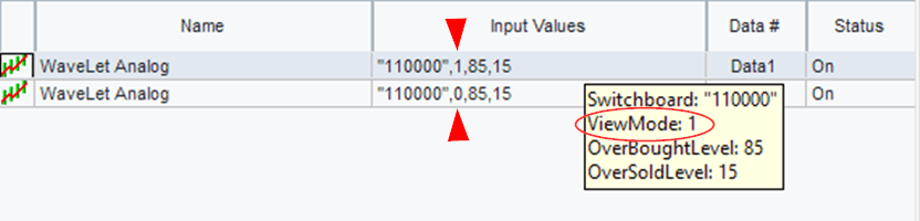
So instead, we sidestep the binary scaffolding while keeping its power by leaning on EasyLanguage’s string-handling capabilities. Rather than six individual toggles, we represent them as a single string of six characters, each a 0 or 1. For example:
“110000”
This string simply means UseD1 and UseD2 are active. You don’t need to know—or care—what the decimal value of “110000” is. A 1 turns on the corresponding UseDX; a 0 turns it off. When more than one 1 appears in the string, the layers are cascaded automatically.
Same analog flexibility. Cleaner interface. Far less friction.
Parsing a string with one simple function: MidStr
Having a nice library of string manipulation functions enforces my prior post on why Quant languages should use the EasyLanguage model. I can easily extract the character at each location located in the string. The first location is represented by one and the last by six.
Here the string is represented by Switchboard and is decomposed by the MidStr function. This function expects two arguments – starting postion and the number of characters to gather. As you can see by the code, we are stepping through each character in the string and extracting that particular character. Based on its value, we integrate that particular layer into the final calculation.
Same math.
Same structure.
Completely different understanding.
One Indicator, Multiple Trading Tempos
Here’s where the iceberg metaphor really matters.
The client had been trading the tip:
- One layer
- One tempo
- One interpretation
But underneath that single line were multiple valid ways to trade:
- Scalpers listening to fast detail
- Swing traders listening to rhythm and rotation
- Trend followers locking onto structure
Nothing was added.
Nothing was optimized.
We just stopped pretending the indicator was simpler than it really was.
The Real Lesson (and Why AI Matters Here)
AI didn’t invent anything in this process.
What it did was help surface alternative ways of thinking — some useful, some not — until the right framing emerged. The insight came from the interaction, not the output.
That’s the part of AI that excites me most for traders.
Not as a signal generator.
Not as a replacement for thinking.
But as a tool for understanding what we already have.
Closing Thought and Nex Steps
Most traders inherit indicators they never fully unpack.
They trade what’s visible and ignore what’s underneath.
Sometimes, the most valuable work isn’t finding something new —
it’s learning how to see what’s already there.
That’s what this exercise reminded me.
In the next installment, i will unpack this intriguing indicator and turn it into a complete trading system.
Final Code and Enhancements
Examples
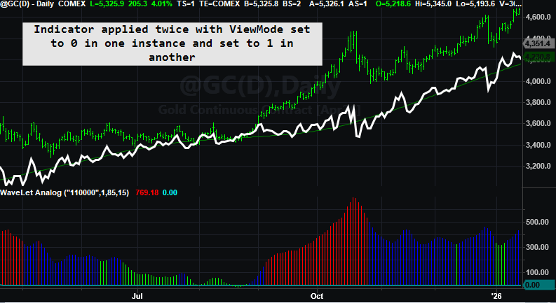
Three charts are shown with three different presets.

Plotting 2 Scales in TradeStation
You can’t plot a single multiple output indicator with different scales in the same chart in TradesStation (well not easily). You have to plot either one or the other and this can be accomplished by using a plot toggle. Here is the toggle in EasyLanguage.