The Throwing-Spaghetti-Against-the-Wall Approach
We now have all sorts of platforms that can test seemingly innumerable combinations of patterns, indicators, trade management rules, markets, and time frames. We have seen systems work on 60-minute bars, but fail completely on 120-minute bars. Popular candlestick patterns are aggressively used to generate systems that pass whatever gauntlet has been defined as “robust.”
The no-coding-required algo generators only look at the metrics. If a system looks great on a 445-minute chart using a HAMMER or HANGING MAN candlestick pattern, and it passes the out-of-sample inline stress testing, then it becomes one of the noodles that sticks to the wall.
I am not being critical of this overall approach. Expanding the search universe by using a wide spectrum of multi-minute bars is somewhat newer, and in many ways, somewhat novel. Back in the day, we mostly stuck with daily bars or common intraday intervals such as 15-, 30-, and 60-minute bars. A 445-minute bar was not even considered. But with today’s tools, almost anything is possible.
What I am critical of is the tendency to take those results at face value without drilling down into the underlying logic. A system that passes a statistical test is not automatically a system that makes sense. And more importantly, it is not automatically a system that can actually be traded.
Enter the Engineer
Plotting the algorithm on the chart and examining the actual trades is Step #1.
Why do this, you may ask? The code is the code. The generator produced an impressive-looking algorithm. The metrics passed the test. The equity curve looked promising.
But what if the algorithm just got lucky? What if it is already drifting away from its foundational premise?
For example, suppose I create a strategy using momentum along with the Hammer and Hanging Man candlestick patterns. The results look promising. A hypothetical generator was fed the available data, churned through the combinations, and produced the following candidate system:
Candidate System
Time Frame: 445-minute bars
Market: @ES
Buy: Momentum is positive and Hammer pattern occurs
Sell Short: Momentum is negative and Hanging Man pattern occurs
Risk: $2,800 to make $5,600
From an engineer’s perspective, I kind of like it.
It has several attractive qualities:
- It is symmetrical.
- It is applied to a good, liquid market.
- It uses a different time frame.
- It involves time-tested candlestick patterns.
- The risk-to-reward ratio is a clean 1-to-2.
But then the engineer asks the next question:
Can the bar interval itself be trusted?
You cannot slice a pie evenly using 30% slices.
Most trading days consist of 23 hours, or:
23 × 60 = 1,380 minutes
Now divide the trading day by the selected bar interval:
1,380 ÷ 445 = 3.10
Or stated another way:
445 + 445 + 445 = 1,335 minutes
That leaves a remainder of:
1,380 – 1,335 = 45 minutes
So, the chart does not really consist of four equal 445-minute bars. It consists of three large 445-minute bars and one small 45-minute bar.
That matters.
A Hammer or Hanging Man pattern detected on a 445-minute bar is not the same thing as a Hammer or Hanging Man pattern detected on a 45-minute cleanup bar at the end of the trading session. The pattern may have the same name, and the code may treat it the same way, but structurally it is not the same event.
This is where generated code becomes engineering work.
The generator saw a metric.
The engineer sees a structural problem

But Can You Argue With the Numbers?
At this point, someone could reasonably say, “Yes, the final bar is shorter, but look at the performance report.”
And that is a fair objection.
The numbers appear impressive. The system produced a solid net profit, a respectable profit factor, and a reasonable percentage of winning trades. On the surface, the strategy looks like something worth pursuing.
But this is exactly where the engineer has to slow down.
Most candlestick patterns are built around the range, body, open, close, high, and low of the bar. In other words, the pattern is not just a label. It is a structural interpretation of price movement during a specific unit of time.
Here is the EasyLanguage definition of the Hammer and Hanging Man pattern:
The key element here is the current bar’s open-to-close body, along with the relationship of that body to the bar’s total range. That makes perfect sense when each bar represents the same amount of market time.
But do you really want to rely on a bar that always covers only 45 minutes when the other bars cover 445 minutes?

From an engineering standpoint, I do not believe the smaller bar provides enough information to fulfill the spirit of the complete pattern. The code may identify the shape, but the market structure behind that shape is not equivalent.
In this case, it appears that a malformed Hanging Man triggered a short sale. The 45-minute cleanup bar completed the pattern, and the system acted on it.
And yet, the numbers look good.
That is the trap.
A performance report can tell you that something worked historically. It cannot tell you whether the logic that produced those trades was structurally sound. That part still requires inspection, judgment, and engineering.

Do You Throw the Results Out Over a Technicality?
Not necessarily.
This is where engineering judgment comes into play. The fact that one of the trades was triggered by a malformed candlestick pattern does not automatically mean the entire idea is worthless. The performance report may still be pointing toward something useful. The combination of market, time frame, momentum filter, and trade management rules may contain real information.
But it does mean the results should not be accepted at face value.
The first question is not, “Did it make money?”
The first question is, “Did it make money for the reason I think it made money?”
That distinction matters.
If a strategy is supposed to exploit a Hammer or Hanging Man pattern, then the bars used to form those patterns should be structurally comparable. A 45-minute cleanup bar sitting next to three 445-minute bars may satisfy the code definition, but it does not necessarily satisfy the trading premise.
So I would not immediately throw the results away. I would move the candidate system into the engineering phase. That means isolating the questionable condition, removing or correcting the structural flaw, and then testing whether the core idea still holds up.
If the system falls apart after making those changes, then the original result was probably more fragile than it appeared. If the system survives, then you may have something more interesting.
That is the difference between throwing spaghetti against the wall and engineering a tradable system.
The generator found a candidate.
The engineer decides whether that candidate deserves to live.
Next Installment — Working Your Craft: Some Coding Required
Don’t worry — I do the heavy lifting for you.
But there is real value in sitting in front of the editor, debugging the code, flipping system components on and off, and examining the functions that drive the trades. That process is a win-win. Even if you do not grasp every minute detail, that is okay.
You do not have to become a full-time programmer to benefit from this exercise.
Understanding the why behind the code is often enough. Why did the trade trigger? Why did the pattern qualify? Why did the system enter there instead of somewhere else? Why did the performance report look good?
Those questions move you beyond blind acceptance of the results. They turn a generated candidate into something you can inspect, challenge, and eventually trust — or reject.
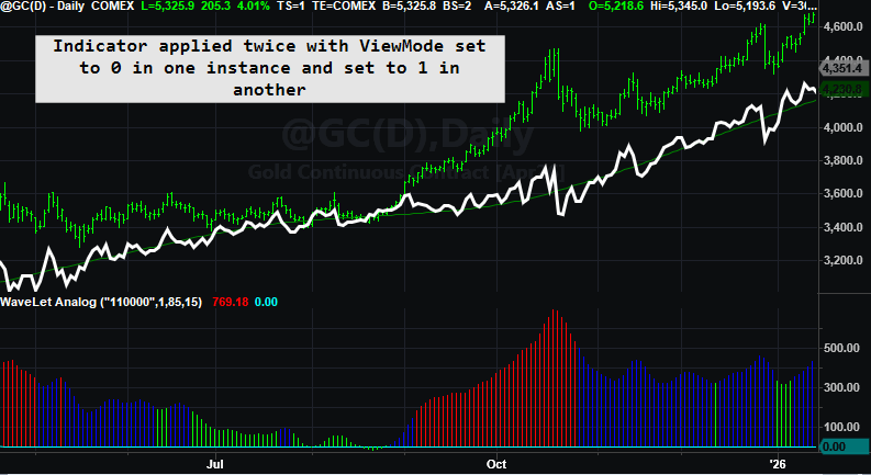
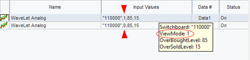
In the next installment, we will take the same strategy idea and make it more practical for real-time trading. The larger bar can still generate the signal, but the smaller bar can handle the execution. In TradeStation terms, Data2 can define the setup, while Data1 handles the trade.
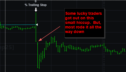
Watching a system trade on a large bar can hide too much of the story. If a trade enters, gets stopped out, or takes a profit all within the same large bar, the report may tell you what happened, but it does not really show you how the trade unfolded.
That is why I like to watch the trade develop on a smaller execution bar. Seeing the five-minute bar crawl across the screen gives you a much better feel for the trade. You can see the entry, the follow-through, the hesitation, the stop pressure, and the eventual exit in a way that a large bar simply cannot reveal.
Maybe that is just me, but I find it much more satisfying.
And more importantly, it provides a clearer picture of whether the trade was realistically executable.
That is where the engineering really begins.